9C, 4D Seismic Processing for the Weyburn CO2 Flood, Saskatchewan, Canada

Abstract

We present a summary of the 9C, 4D processing used for the seismic monitoring of a CO₂ flood in the Weyburn Field, Saskatchewan, Canada. The resultant time-lapse amplitude anomalies for both the P- and S-wave volumes are coincident with the locations of the CO₂ injection patterns. Furthermore, the anomalies we observe are robust in the sense that they persist from the preliminary brute stacks through to the final processed images. We believe this is largely due to the high degree of repeatability of the monitor surveys. We used a twenty-meter cutoff (one half of the group interval) with regards to similarity of source and receiver locations between the monitor survey and the baseline surveys. Ultimately, we edited 7% of the shots due to positioning errors. The primary prestack processing steps include appropriate shot and receiver edits, source- and receiver-related phase corrections (and reversals), independent refraction statics, common velocity models (between baseline and monitor), independent residual statics, and a common pilot for trim statics. A post-migration cross-equalization algorithm is used prior to analysis of the differenced volumes.

Geological Setting and Production History

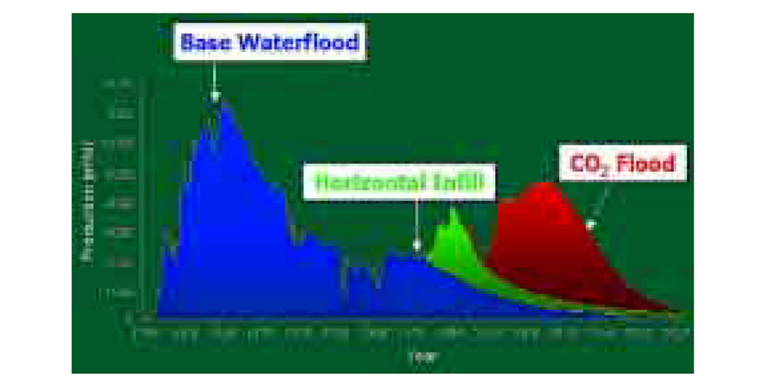
The Weyburn Field is located on the northeast flank of the Williston Basin in southeast Saskatchewan, Canada (Figure 1). The field was discovered in 1955 and conventional production progressed to waterflood recovery 10 years after discovery (Figure 2). Approximately 1000 wells, including 137 horizontal wells with 284 lateral legs, have been used to recover 24% (primary depletion and conventional waterflooding) of the 1.4 billion barrels of oil originally in place. EnCana, the field operator, initiated an enhanced oil recovery project (CO₂ miscible flood) in October of 2000. Initially, 19 horizontal well patterns were converted to CO₂ injection with injection rates of 3 to 7 mmcf/day/well. It is anticipated that this project will recover an additional 15% of the original oil in place. The CO₂ flood is designed to target the unswept reserves in the upper Marly unit of the reservoir.

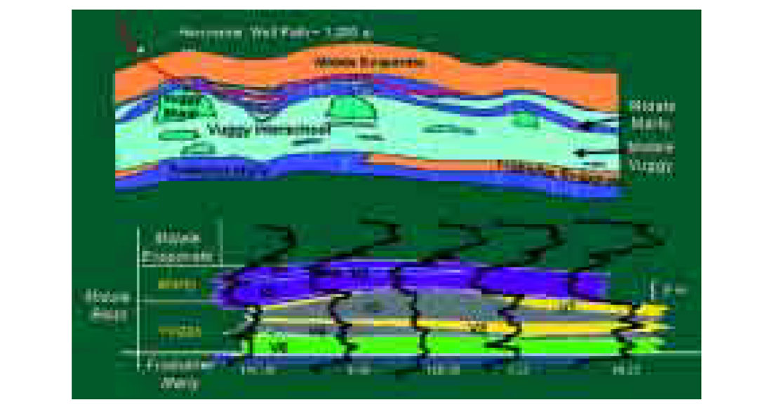
The Midale carbonate reservoir consists of two distinct zones at a depth of approximately 1450m (Figure 3). The upper Marly unit has low permeability of approximately 10 md, high porosity, averaging 26%, and ranges in thickness from 7-10m. Horizontal wells drilled since 1991 in Weyburn Field have targeted the Marly as a zone of bypassed pay. These wells have substantiated the belief that the Marly unit was not as effectively swept as its underlying counterpart, the Vuggy. The Vuggy averages 15 md permeability and 11% porosity and ranges in thickness from 15 to 20 m. The flow capacity of the formation is the product of permeability and net thickness from both the Marly and Vuggy. The Marly has a low flow capacity relative to the Vuggy and correspondingly low sweep efficiency. The potential for recovering bypassed oil in the Marly is greater with CO₂ flooding than it is with water flooding because of the comparatively high mobility of CO₂.

9C Acquisition Design For Seismic Monitoring

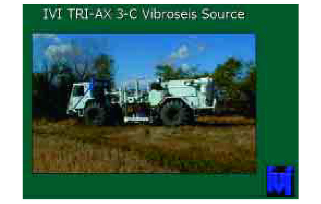
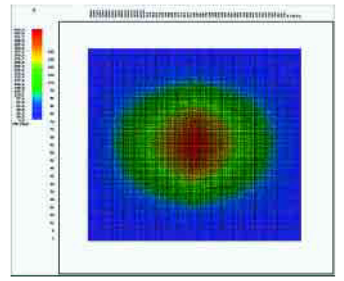
To assist in monitoring CO₂ flood performance, a timelapse (4D), multicomponent (9C) seismic monitoring project was implemented by the Reservoir Characterization Project (RCP) at the Colorado School of Mines (CSM). The 4-D, 9-C seismic surveys at Weyburn were designed for a uniform azimuth and offset distribution and to provide high-resolution coverage over four CO₂ injection patterns. During the acquisition of the monitor surveys, all efforts were made to occupy the same source and receiver locations. The initial baseline and two subsequent monitor surveys were acquired in the fall of 2000 (prior to CO₂ injection), 2001 and 2002 respectively. Because the reservoir is thin relative to the seismic wavelength it is necessary to use seismic amplitudes rather than time delays in order to monitor changes in the reservoir. Therefore, the survey was designed for high spatial sampling, density and fold. Useable pure-mode fold is approximately 400 (Figure 5) in the middle of the survey for P-wave data and 140 for S-wave data. The data were acquired using triaxial vibroseis sources that allow for expeditious 9C acquisition of the three source components; one vertical and two orthogonal horizontal displacement modes (Figure 4). The source-line interval was 80m, with a source interval of 80m at the edges of the survey and 40m near the center. In the vertical mode, three sweeps of 8-180 Hz over 10 seconds with a 4 second listen time were used (14 second record length). In the horizontal mode, four sweeps of 6-80 Hz over 10 seconds with a 6 second listen time were used (16 second record length). There were 28 source lines with 33 or 66 sources per line. Bunched 3C (3X3C) geophones were used with a receiver-line interval of 140m and a group interval of 40m. There were 20 receiver lines with 60 groups per line.

Rock and Fluid Physics Modeling

In addition to the repeatability of the acquisition phase of the project, 4D data processing is another critical part of the overall success of timelapse analysis and ultimately CO₂ detection. As suggested in rock and fluid physics measurements and modeling, the addition of CO₂ to the system would cause a 4-6% decrease in P-wave velocity with a corresponding 15-20% change in reflection amplitude. These results were considered optimistic as the rock physics work suggested the Marly would experience the greatest changes due to its high porosity but it is also the thinnest unit in the reservoir. Shear-wave velocity modeling suggested that in the fracture zones, interval shear velocity-anisotropy (HTI) could change by 5-10%. The high interparticle or pinpoint porosity in the Marly suggests that the P-waves should be more sensitive to changes in that unit. Whereas, the fractures and channel porosity fabric in the Vuggy may be more detectable on the shear-wave data. In light of these predicted small changes in velocity and because the reservoir is thin relative to the seismic wavelength, it was presumed that seismic amplitudes would be most applicable for the detection of changes in the reservoir due to CO₂ injection. Therefore, the primary processing objective was to preserve relative amplitudes between the baseline and monitor surveys. All components were processed to preserve the consistency between surveys and to enhance the timelapse analyses of the data. The excellent data quality, high spatial sampling and high fold helped facilitate the use of surface consistent linear processes which are designed so that true-amplitude analysis can be done. Note reservoir factors such as noise interference, acquisition and processing artifacts and insufficient resolution could easily mask the subtle 4D signals.

9C 4D Processing

The two most important steps in the processing of the Weyburn 9C, 4D data were the horizontal source and receiver polarity corrections and the shear-wave statics. Other key processing considerations were:

1. Editing of bad or mispositioned shots and receivers.
2. Independent computation of weathering statics due to varying ground conditions between the monitor and baseline surveys.
3. Identical velocities for repeat surveys as determined from the monitor survey.
4. Separate residual statics.
5. Common pilot traces for the trim statics as determined from the monitor survey (P-wave only).
6. Prestack phase and bulk static corrections for different sources.
7. Post migration cross-equalization and differencing.

After common geometries were written, shot and receiver editing was done to remove locations either not occupied for all three surveys or, in the rare case, where the locations were deemed too far apart. The final edits resulted in approximately 7% editing of sources and less than 1% for the receivers. The primary reason for not being able to occupy the same location was due to the wet ground conditions during the baseline survey in 2000. For the monitor survey in 2001, the ground conditions were exceptionally dry and for the second monitor survey in 2002, the ground was frozen. Therefore, it was necessary to calculate refraction statics independently for the two surveys. The three vintages of data are reasonably similar with respect to data quality, yet the 2002 vintage has the best signal to noise characteristics. Independent velocities were picked for the three surveys and they were nearly identical. This fact and the overall data quality on all three surveys allowed us to use the velocities and mute from the baseline survey. Residual statics were calculated independently.

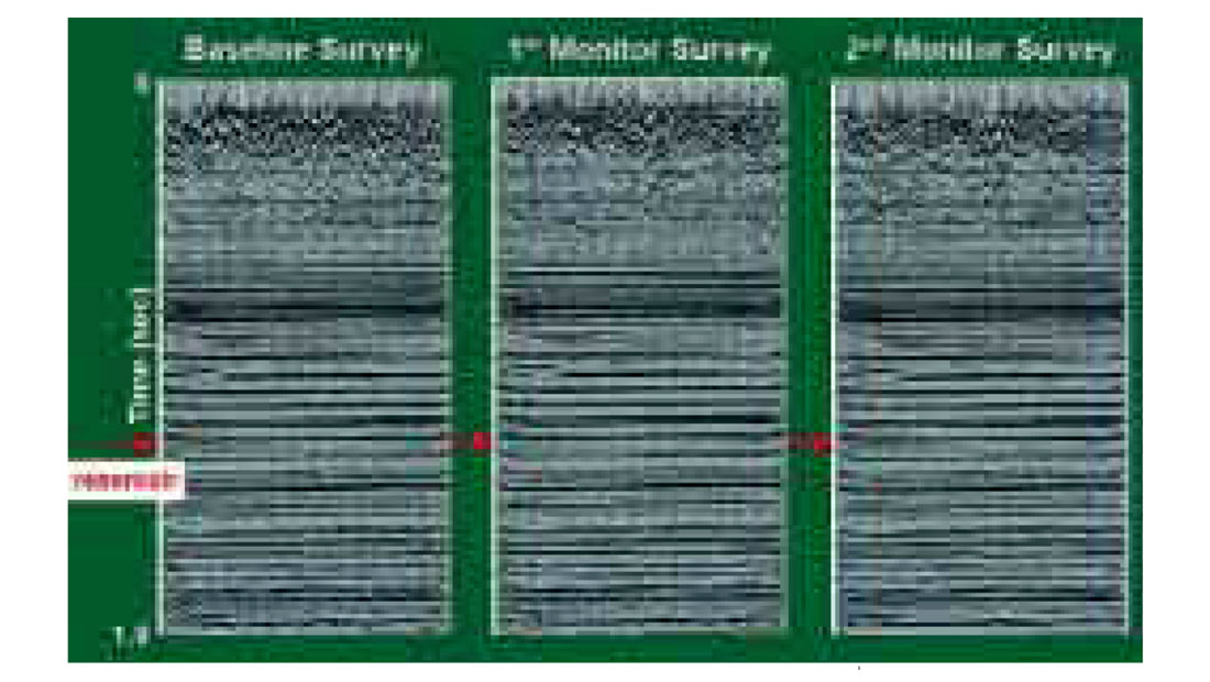
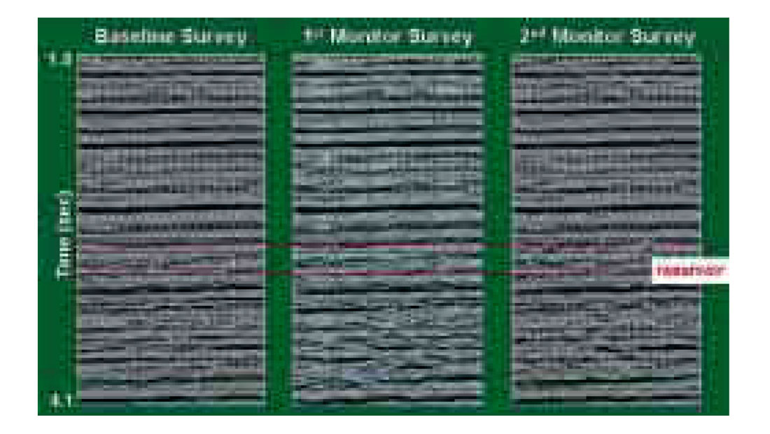
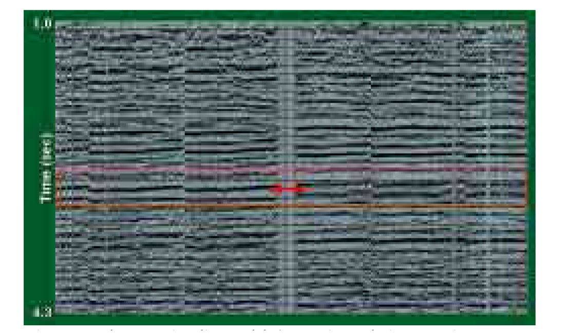
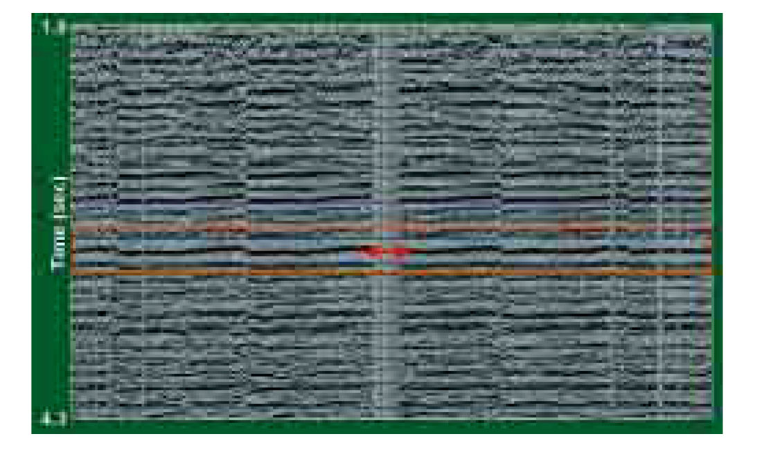
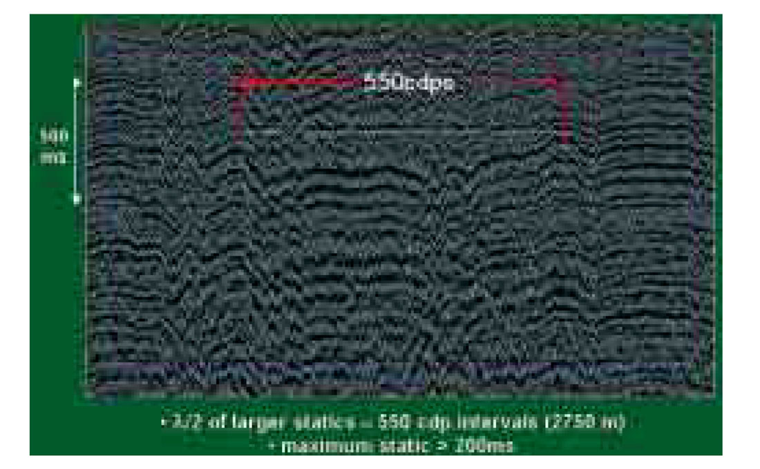
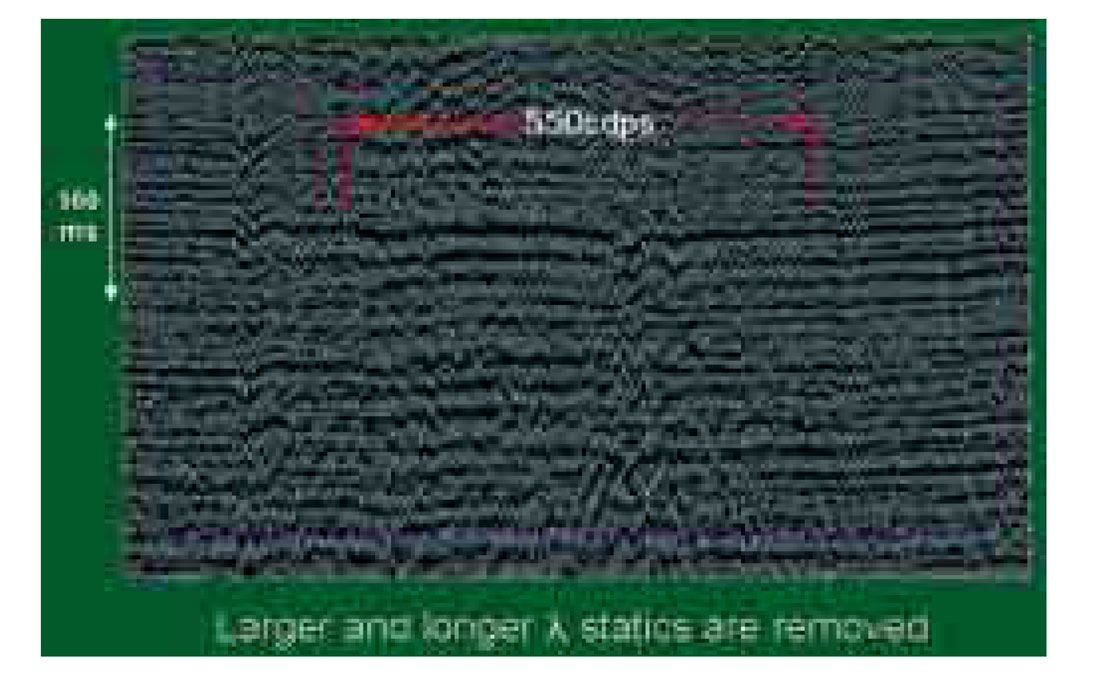
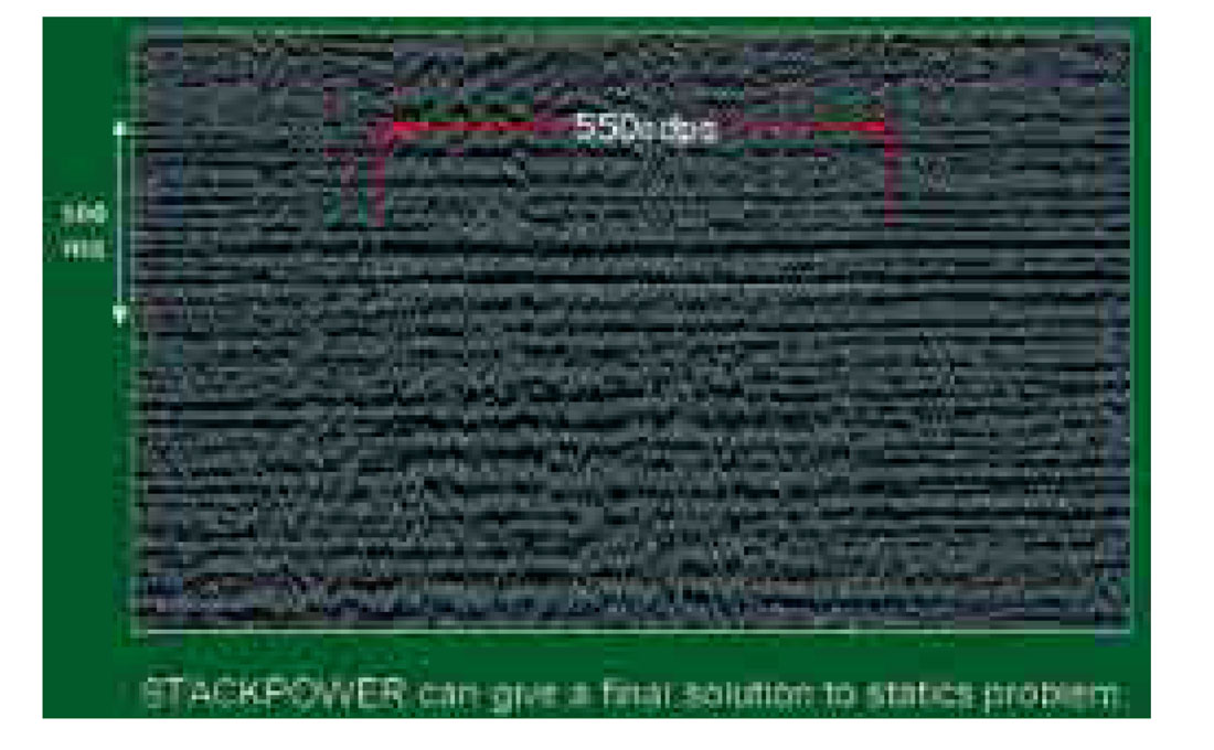
Phase analysis of the shot stacks revealed a difference at the edge of the survey (4 source lines). It is not exactly clear what caused these differences. However, the difference (approximately 85 degrees) was accounted for and velocities and residual statics were rerun. The final prestack process was a trim static that is calculated using a common pilot that was derived from the 2000 vintage data. The volumes were then stacked and migrated. The final step, before analysis of the differenced volumes is a cross-equalization process that accounts for phase, static and amplitude differences on a trace-to-trace basis (Figures 6-8).

The P-wave and S-wave processing flows are nearly identical. However, the S-wave data is comprised of four volumes after Alford rotation (S11, S12, S21 and S22). The S11 and S22 or principal components are processed independently with different velocities and statics. The S12 and S21 or off-diagonal components are processed using an average of the velocities and statics from the main diagonals. Residual rotation analysis can be done at this point. Due to the reduced signal to noise ratio on the S-wave data, a prestack noise attenuation process (Radon-based) was applied in the shot domain. This step was not necessary for the P-wave processing.

Horizontal Source and Receiver Polarity Reversals

One of the major steps during the processing of the Weyburn dataset was correcting for errors in the receiver and source polarizations (polarity reversals). The PS data were used to correct for receiver polarization issues and the Alford-rotated SS data were used to correct for source polarization errors. We used a mid-range limited-offset linear move out correction (LMO) on the first breaks to form a first-break LMO receiver stack. It was not until the timelapse (first monitor survey) data were available that we were able to clearly identify the problem. However, once we saw the inconsistencies in the timelapse analysis, we were able to identify and correct for the polarity reversals for each of the three surveys (Figures 9,10). The source-side polarity reversals were then identified using a similar approach. That is, we used a mid-range linear-offset LMO correction to create a shot stack and then looked for polarity reversals in a timelapse and shot-line sense (Figure shot reversal). These corrections to receiver and shot polarizations were the single most important processing step.

S-wave Statics

Shear-wave statics are often very large and not related to p-wave statics (Figure 11). In fact, due to differences in P-wave and S-wave velocities and hence travel times through the weathering layer (largely due to water saturation in the weathering layers), S-wave statics can be an order of magnitude greater than P-wave statics (Figure 11). Shear-wave first-break refraction statics are often difficult to characterize due to near-surface inhomogeneities and anisotropy. In order to get to the pure-shear statics, we first had to solve for the pure-compressional statics and use the source term from that as a starting point for the PS statics. Once the PS statics were solved (Figures 12-14), we mapped the receiver term to the source and receivers of the pure shear modes. We then used residual statics and trim statics independently for the S1 and S2 modes.

Preliminary Data Analysis

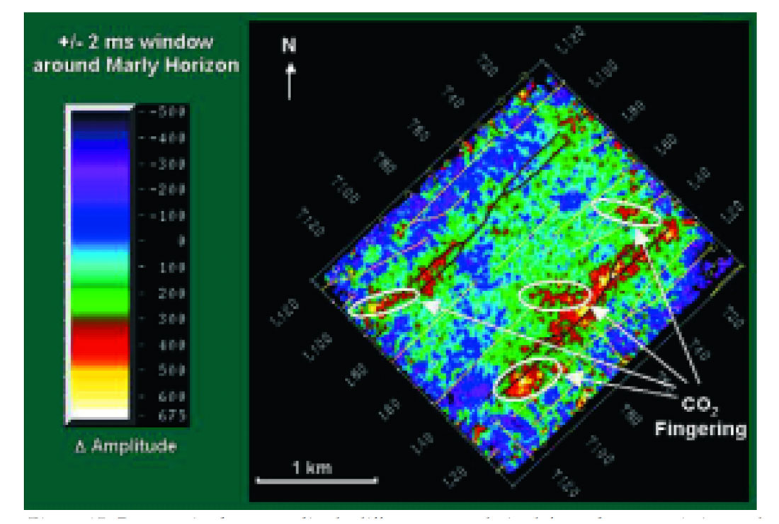
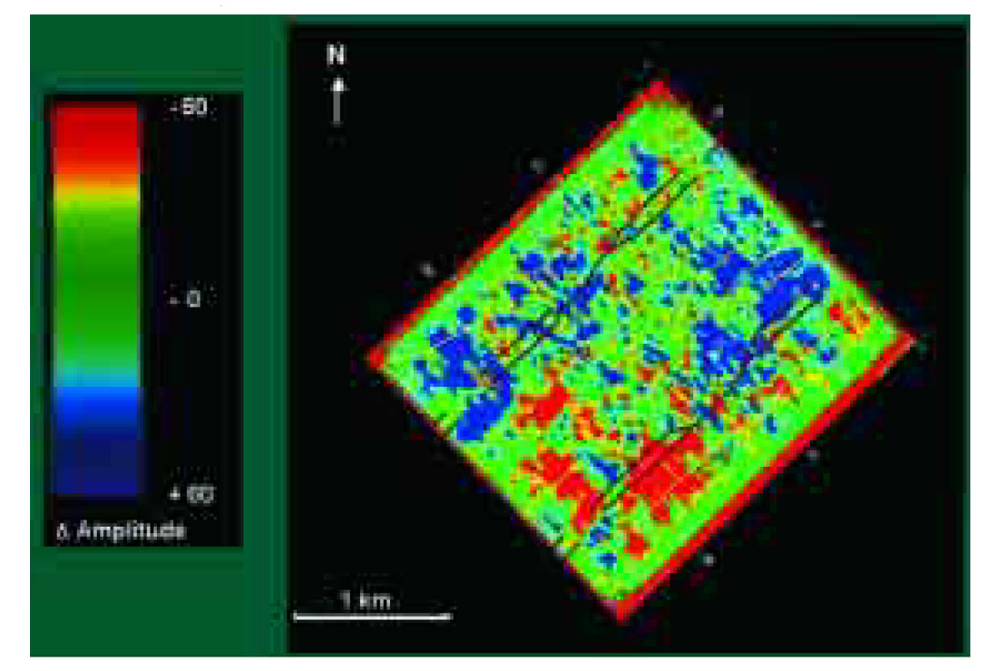
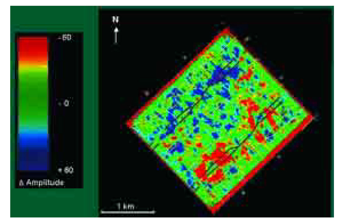
While a full discussion of these results is presented in another paper (Davis et al, 2003), we do include selected time slices of the final volumes. A more accurate representation of the anomalies is possible using horizon-based amplitude extraction of the final differenced volumes. Figure 15 is an amplitude extraction of the differenced volumes (baseline minus first monitor) at the reservoir level, oriented to north and showing the horizontal injector and producer locations (Figure 15). The three-injector patterns that show the strongest anomalies correspond with the injectors that had the most CO₂. The southern pattern had five times as much CO₂ as the northern one. Figures 16 and 17 show a time slice of the final differenced S1 and S2 volumes respectively. While the P-wave and S1 volumes exhibit similar trends, the S2 additionally shows the subtle development of a perpendicular trend, perhaps suggesting a sensitivity to the presence of fractures (see Davis et al, 2003 and Li, 2003).

Conclusions

We have presented a summary of the 9C, 4D processing flow used for the analysis of a CO₂ flood in the Weyburn Field. The robustness of the timelapse analysis was largely assisted by the acquisition design and the similarity of the source and receiver locations for the two surveys. The true amplitude processing approach has allowed for the detection of subtle amplitude anomalies in very good agreement with the reservoir production model and production/ breakthrough data.

The two most important steps in the processing of the Weyburn 9C, 4D data were the source and receiver polarity corrections and the shear-wave statics.