Depth Conversion and Seismic Lithology Inversion of a McMurray Oil Sands Reservoir

Summary

The Lower Cretaceous McMurray Formation in NE Alberta is a prolific oil sands reservoir. In Statoil Canada Ltd. Leismer leases, about 100 km south of Fort McMurray, the bitumen saturated reservoir lies at a depth of approximately 450 m with SAGD (Steam Assisted Gravity Drainage) being the optimal method for production. The cost intensive SAGD operation requires a detailed mapping of the subsurface. This paper discusses two aspects of the seismic based subsurface interpretation: Depth conversion and Seismic lithology (sand-shale) characterization.

The statistical approach for depth conversion not only demonstrates that the reservoir depth can be predicted with high accuracy but also that reliable uncertainty estimations can be provided. The lithology characterization, which is based on pre-stack seismic inversion and neural network inversion, yields seismic volumes of gamma ray and porosity. The combined interpretation of the PSTM (PreStack Time Migrated) seismic volume and the inverted volumes allows for a detailed interpretation of the oil sand reservoir. This approach to subsurface reservoir interpretation leads to an improved placement of horizontal wells and a reduction in a number of required vertical delineation wells.

Introduction

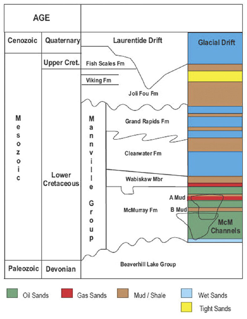
The study is based on data of the McMurray Formation reservoir in Statoil’s Leismer assets in NE Alberta (figure 1). The McMurray Formation represents a fluvial estuarine depositional system, hosting rich bitumen and water-sand reservoirs. The general stratigraphy is shown in figure 2. The unconsolidated sands of McMurray Formation within the Leismer are in at depth of about 450 m, with a pay thickness of up to 40 m and porosity between 27 % to 30 %. The sands are inter-bedded to varying degrees with muds. Depending on the depositional environment the muds can be localized or extend over large regions.

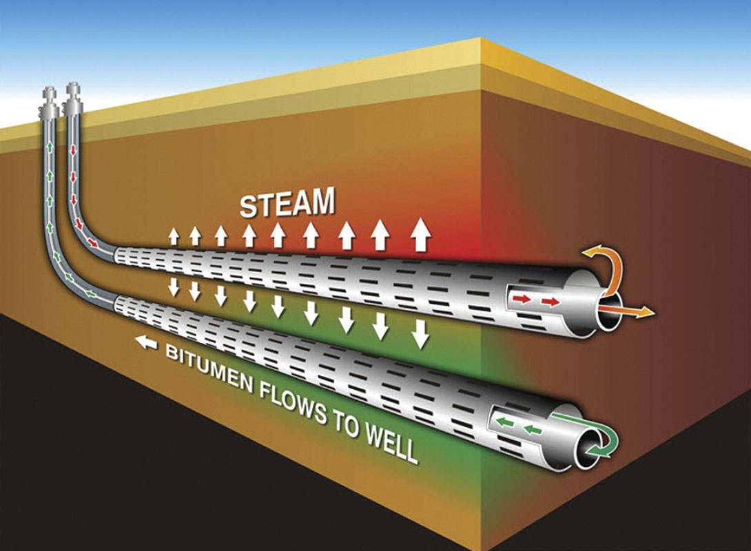
SAGD, the production method of choice, uses horizontal well pairs to extract the bitumen. The upper horizontal well is for steam injection and the lower well for oil drainage (figure 3). Compared to “conventional” mining of oil sands this method has a much smaller surface footprint. However, SAGD can be operated efficiently only if the subsurface geoscientist team is able to image/model/predict the subsurface with high accuracy. Knowledge of the depositional facies, geometry of the reservoir, including top and base of the SAGD pay interval, and thickness, distribution and lateral continuity of potential mud baffles and barriers are critical for a successful SAGD operation. The challenge for subsurface imaging is the high degree of reservoir heterogeneity.

One means of optimizing SAGD well-pair performance is to place the producer well as close as possible to the base of pay. The actual optimal distance depends on the nature of the base of pay, i.e., if we deal with bottom water the producer well offset from base pay (i.e. bitumen/water contact – BWC) is greater than for a base of pay defined by the Devonian carbonates unconformably underlying the McMurray Fm. Communication between the injector and producer is essential, so SAGD well pair placement favors reservoir facies which do not have permeability barriers enabling optimal production. Only reservoir above the production well will be drained, therefore, every meter closer to the base reservoir could translate to an additional one million barrels accessible per well pad. Consequently, an accurate depth conversion is critical.

In the Leismer area Statoil Canada owns more than 75 km² of 3D seismic. The 3D survey defines the outline of the study area. Within the 3D seismic area more than 150 wells existed prior to 2010 and more than 60 additional wells were drilled during the 2010 winter season. Due to the very high well density, the analysis of well data alone allows for the creation of a good starting model of the subsurface. Ideally, cost savings can be achieved and reservoir characterization improved by using seismic to accurately resolve inter-well areas; therefore, seismic based mapping becomes vital. Two aspects of the geophysical interpretation, depth conversion and seismic sand-shale characterization, are discussed in this paper.

Depth Conversion

Accurate depth conversion assures that the SAGD well pairs can be appropriately placed close to the base of the reservoir allowing for an optimal drainage of the reservoir. The first step in depth converting the reservoir zone is to create a robust frame, i.e., to pick reliable horizons close to the top and base of the reservoir. In our case the most reliable picks were the Wabiskaw Formation top and the Devonian top surfaces. The impedance contrast is in particular strong for the Devonian top surface, which is the interface between the clastics of the McMurray Formation and Devonian carbonates. This results in a strong consistent seismic phase. In general this phase can be automatically picked with the exception of a few areas, where the seismic phase splits into two events due to karsting. The Wabiskaw Formation top is the interface between a sandy Clearwater Formation interval and the shale dominated Wabiskaw Formation. The seismic phase is not as consistent as the Devonian interface because of the varying sand-shale content. After careful picking in the time domain, the depth conversion of the bounding surfaces is optimized, then the intra reservoir horizons are scaled between the boundaries. In an area with more than 150 wells within the 3D seismic area, approximately 2 wells/km², a statistical depth conversion using kriging and simulation techniques becomes the method of choice. The velocities in the study area do not show any depth dependence, but the lateral variation is considerable. Local shallow channels create velocity anomalies which have to be captured for an accurate depth conversion. The statistical depth conversion can take care of local velocity anomalies.

Acknowledging the lack of depth dependence of the velocity field, the following strategy was applied for a successful depth conversion:

• Build floating datum (FD).
• Establish the velocity field between FD and Wabiskaw or Devonian time picks and their corresponding well picks (in depth) at the well locations.
• Krig the velocity field
• Create a depth surface for Wabiskaw and Devonian
• Convert intra McMurray Formation horizons including top and base oil sand reservoir using a linear depth interpolation between the Wabiskaw and Devonian horizon.

Alternatively, a layer cake approach was tested which included the shallower the Grand Rapids Formation pick. The layer cake model did not improve the reliability of the depth conversion.

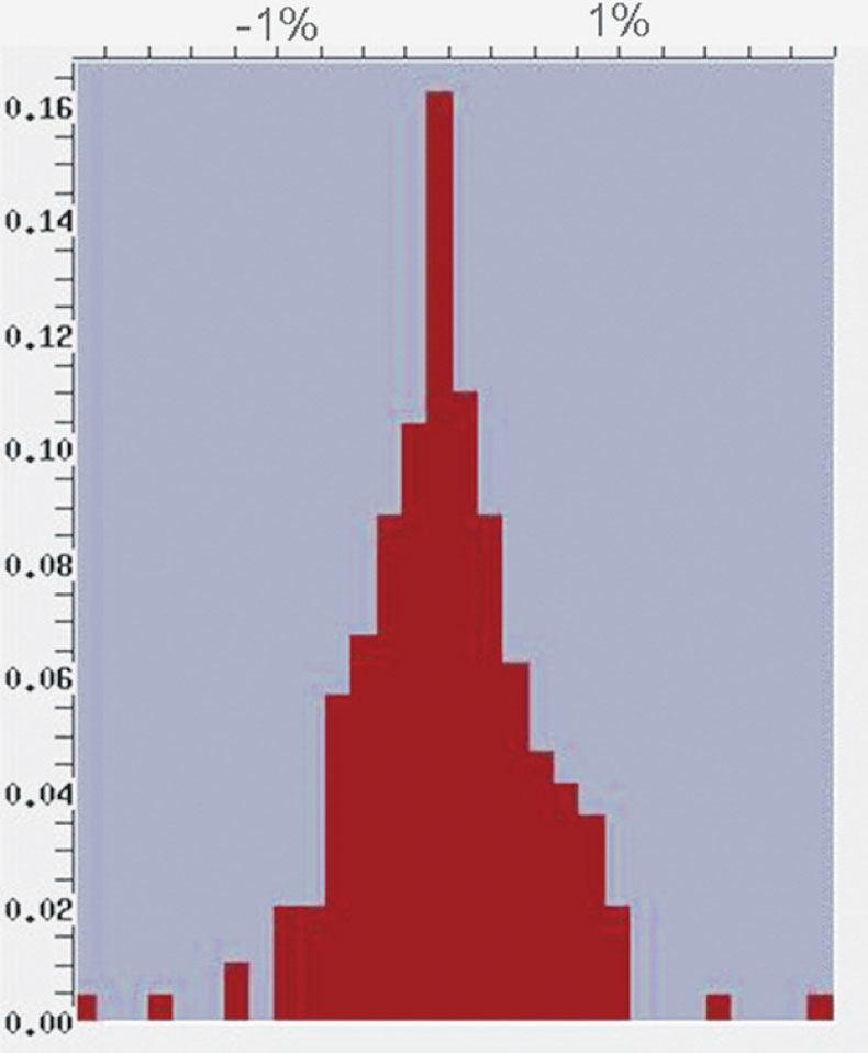
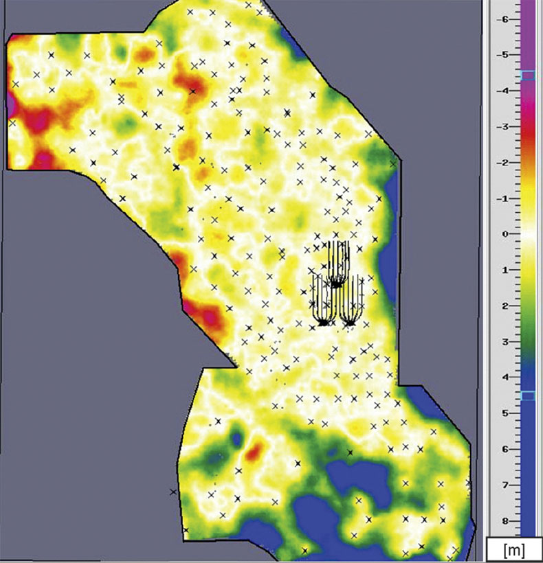
An advantage of statistical depth conversion is the simplified evaluation of uncertainty. Cross validation allows for studying the impact of individual wells on the kriged solution. Figure 7 shows the histogram of the cross validation error at the well locations. The velocity histogram indicates a standard deviation of 0.5%, which translates into a depth error of +/- 2.3 m. Sequential Gaussian Simulation helps to understand the uncertainty between wells, i.e. how much can we bend the surface up or down without violating the statistics and keeping the well-ties fixed. The results indicate that the depth prediction error to the base reservoir horizon in the densely drilled study area is less than 1.5 m (figure 8).

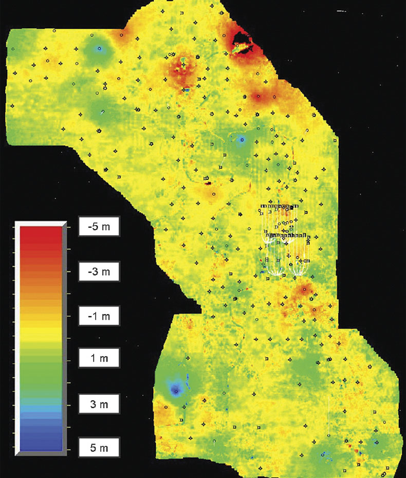
After the depth conversion was finished more than 60 additional wells were drilled within the 3D survey area. The average depth error was close to zero, which implies that the depth conversion was not biased to the positive or negative side. The average absolute error was 1.6 m for the Wabiskaw surface and 1.4 m for the Devonian surface. This average absolute error is more critical and demonstrates not only the robustness of the depth conversion but also the validity of the statistical error analysis. Figure 9 shows the difference of the Devonian depth conversion with and without the new (2010) wells. The larger errors in the NE corner of the survey resulted from a local mis-pick of the Devonian time horizon, which was corrected after drilling a key well.

Seismic Lithology Inversion

A successful SAGD project depends on the quality of the reservoir sand. Relatively minor facies differences between sandy or sandy/shaly inclined heterolithic stratification (IHS) and estuary sand can make a significant difference in the production (Strobl, 2010). Also, thin but continuous shale or mud layers can impede the development of steam chambers and the subsequent drainage of mobilized bitumen in the SAGD process. Therefore, the mapping of reservoir quality and the heterogeneities is critical. Seismic can significantly support this mapping. Before evaluating 3D seismic attributes, the analysis of log attributes illustrates the feasibility of using seismic to predict lithology.

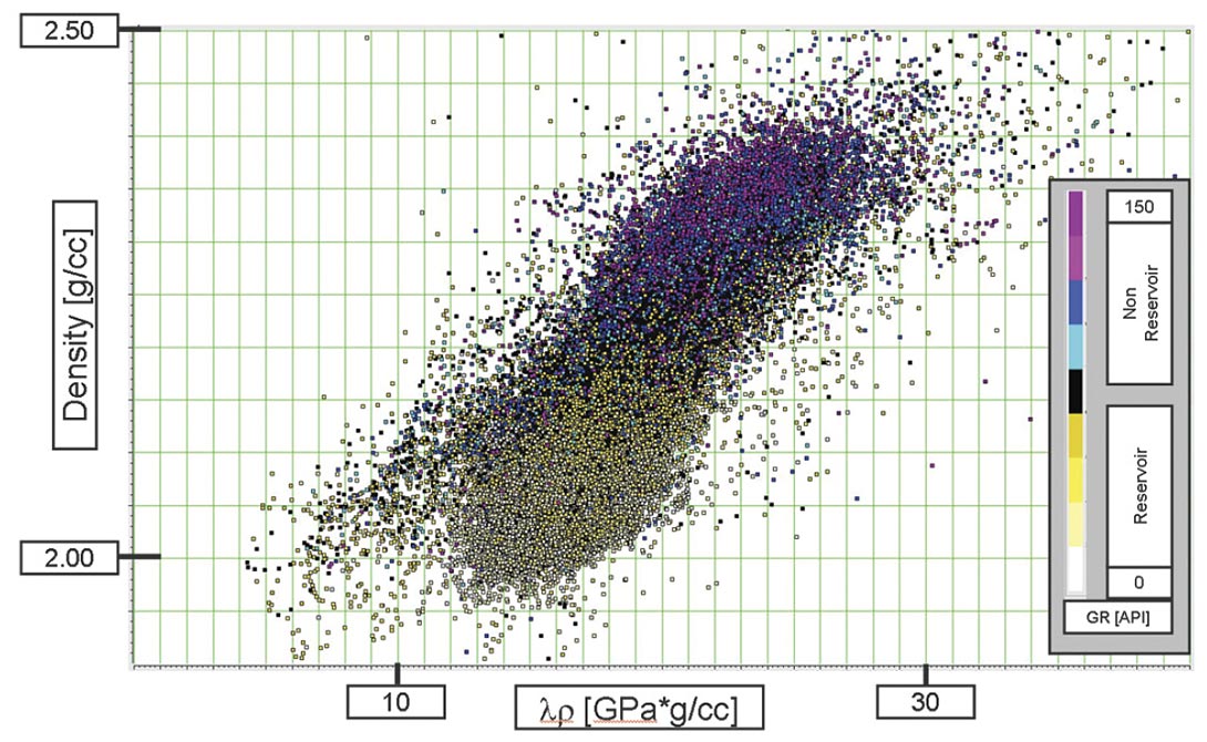
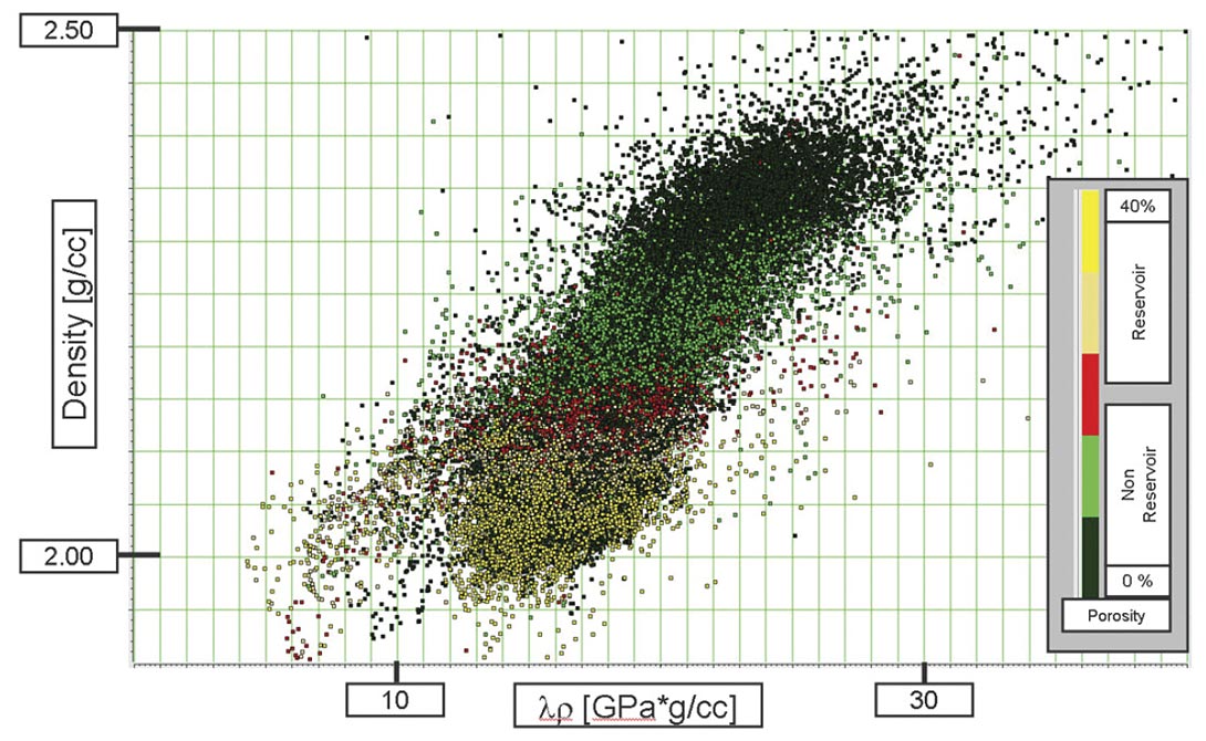
It is well known that density correlates to reservoir properties like gamma ray or shale volume, e.g., Xu and Chopra, 2008; or Bellman, 2007. Multi dimensional correlations are even more pronounced. Derived from log data the cross-plot in figures 10+11 illustrate that density and lambda-rho are powerful attributes for gamma ray or porosity classification. Please note: λρ was chosen as the log attribute, because λρ can be directly extracted from a prestack inversion of seismic data. The coloring of the data points is based on cut offs between reservoir and non-reservoir. The attempt to correlate water saturation and seismic log attributes looks promising in figure 12, however, the situation is complicated by the fact, that this cross-plot shows more a sand – shale dependency than a water saturation dependency. A robust definition of the bitumen saturation or the bitumen-water contact from seismic attributes is still under evaluation.

Dumitrescu (2008) showed that density can be extracted from 3D surface seismic data using a neural network approach and infers the reservoir top and base from the density. Xu and Chopra (2009) discussed a three term inversion approach for reliable density interpretation and continue with a linear transformation to derive gamma ray and shale volumes from density. In contrast, this paper discusses a workflow which uses the results a 3 term inversion in a neural network to invert for reservoir parameters like gamma ray and porosity.

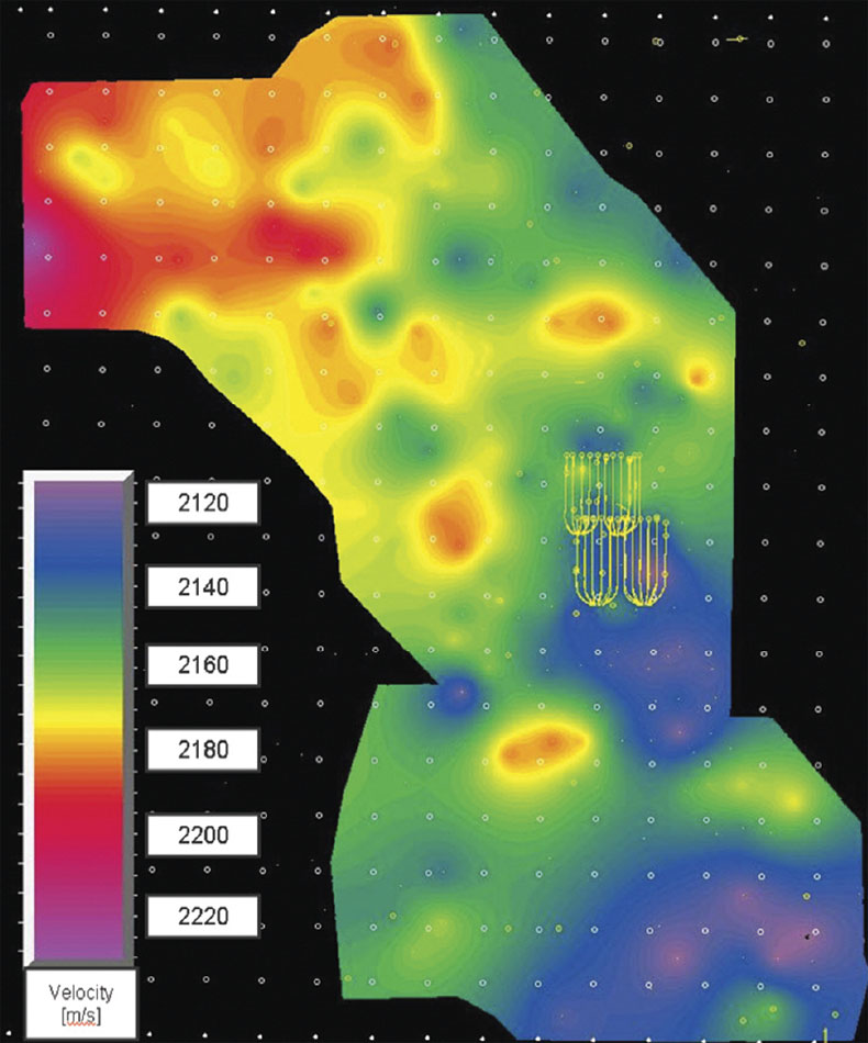
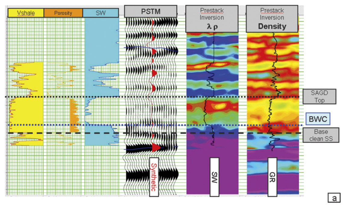
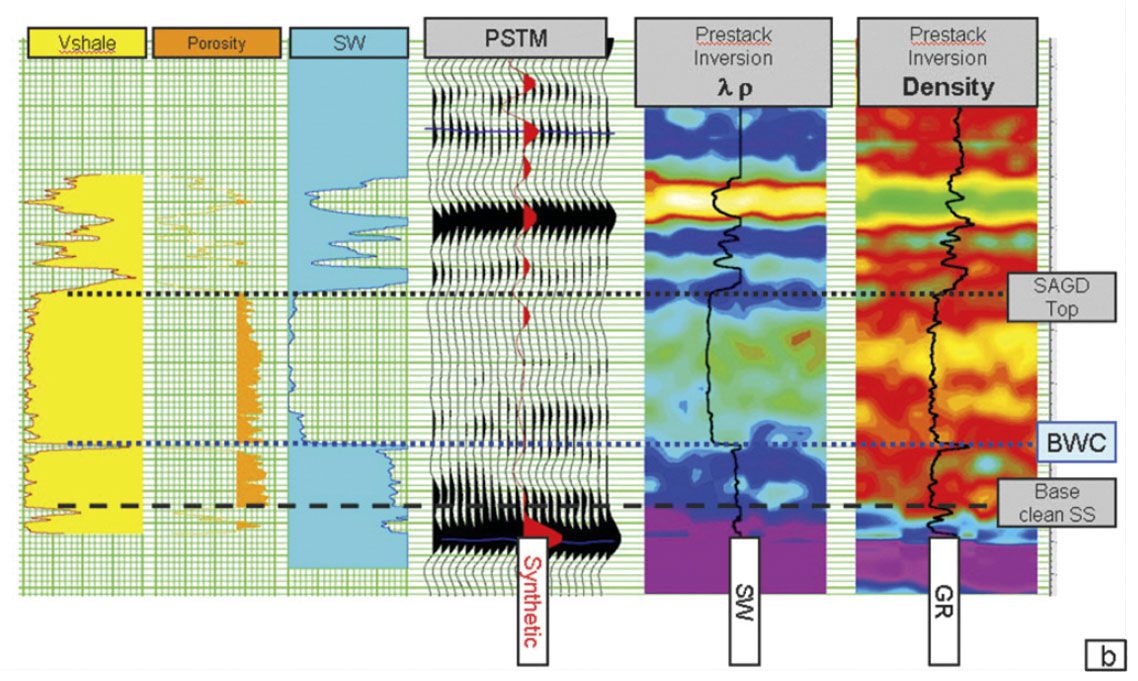
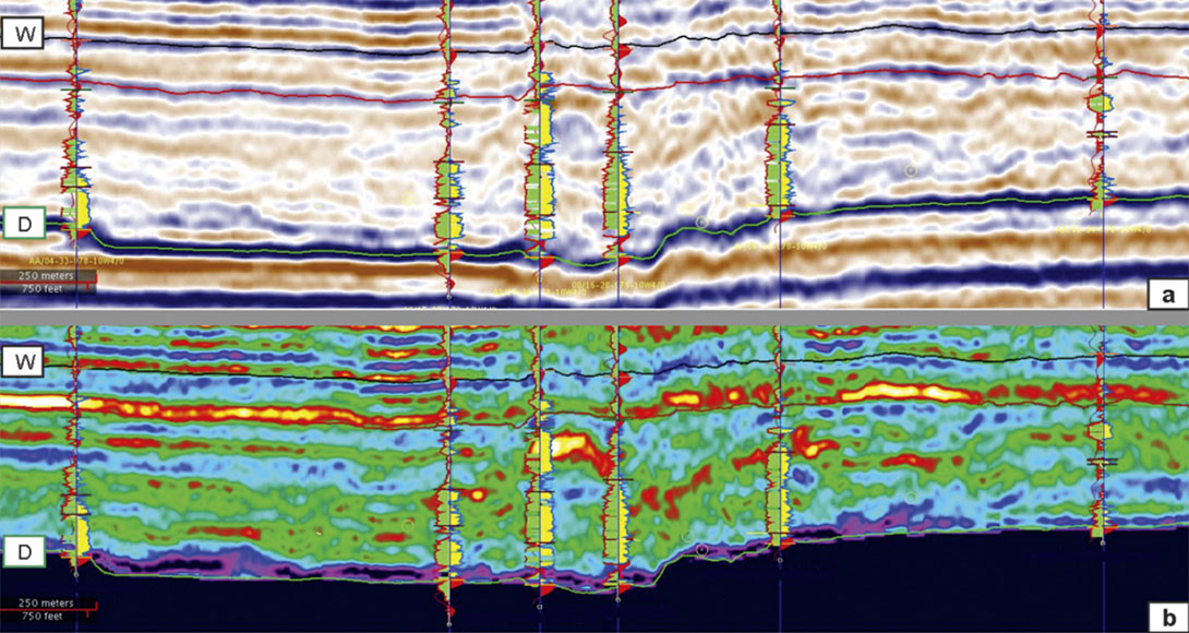
After careful AVO compliant processing of the 3D survey, prestack inversion delivered reliable results for seismic reservoir characterization. The well tie in Figure 13a shows the strong correlation between reservoir parameters and inversion results. To emphasize the correlation, the SW curve was inserted into the λρ section and the GR curve into the density section. Unfortunately, not all well ties are of this excellent quality for two reasons: firstly, well ties within the reservoir zone are frequently poor already for stacked data, and secondly, inversion results are not always stable. Figure 13b illustrates a poor synthetic seismogram to PSTM tie but still a reasonable SW-λρ or GR-density tie. Additionally a number of well ties exist with poor ties in any domain. We cannot trust absolute numbers but the trend is robust. Figure 14 shows the PSTM section (a) and the inverted &lambada;ρ section (b) through several wells. The location of the section is shown in figure 16. On this line not only the bright response of a gas filled sand (center wells) can be detected but also a reasonable correlation to the gamma ray logs (in green) and porosity (in yellow) logs is visible.

The seismic interpretation of reservoir quality can be even better facilitated with a neural network inversion for parameters like gamma ray or porosity. In a supervised neural network training process using a probabilistic neural network, seismic attributes are combined and inverted to reservoir parameters. For this purpose a limited set of seismic input attributes is selected based on their sensitivity to the output reservoir parameters. Between four and seven attributes were chosen and combined in the neural network inversion. Quality control is the most important step in the neural network inversion. Only cross-validation or true blind tests can prove the reliability of a neural network prediction. With close to 200 wells within the 3D survey, the training of the neural network can be done on a small fraction of the data only. In this specific case only approximately 10% of the well data base was used for training, the remaining 90 % are potential candidates for true blind tests. Figure 15a, which shows a section with gamma ray inversion, and Figure 15b with the corresponding porosity inversion, proves the high quality of the inversion process. The inserted logs are gamma ray in green and porosity in yellow. All the inserted wells are true blind tests, i.e. they were never part of the training. As can be seen from the well on the right hand side of the section, not all wells exhibit a perfect tie, but in most cases the inversion can guide the interpreter very well. Porosity or gamma ray boundaries can be impressively illustrated with the correct color bar selection, but details have to be worked out by the interpreter. The author’s strategy is viewing the PSTM section and several inversions simultaneously; this allows deriving a detailed interpretation.

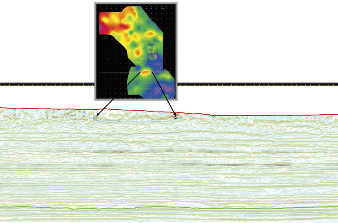
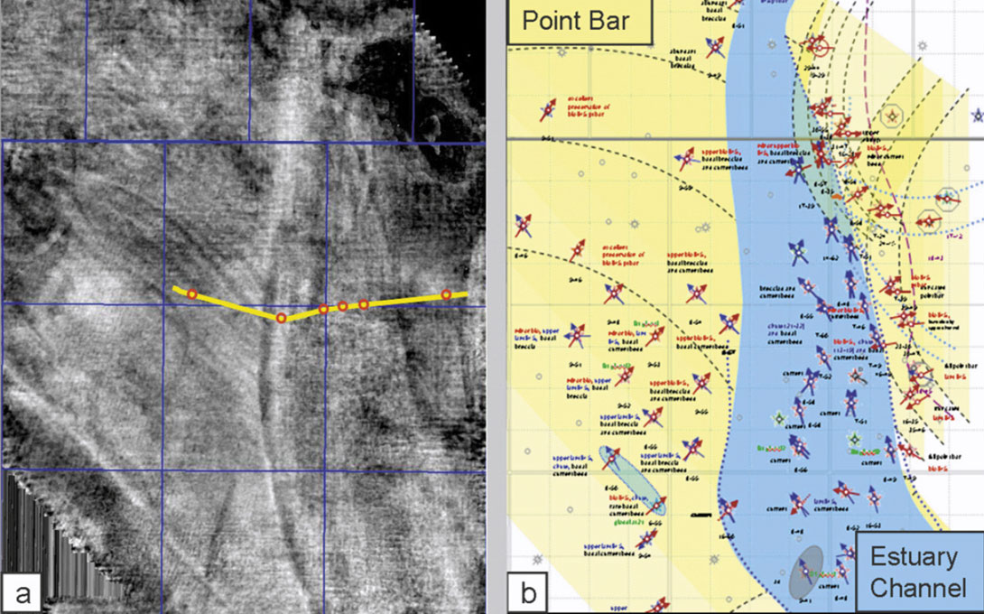
In most cases it is very challenging to follow individual sand or shale channels throughout the 3D volume. This process can be supported with the interpretation of time slices, in particular, slices through inverted volumes. Figure 16a shows a time slice through the λρ volume, which cuts through the reservoir section. A number of linear and curved features can be recognized. In particular curved elements can be identified in the NW area and a long NS feature of low contrast, which is bounded by strong reflections. These features correlate very well with independent interpretation of High Resolution Micro Imager (HMI) log data shown in figure 16b. H. Brekke (Statoil’s internal report) interpreted the blue area as the main estuary channel and the yellow area as a point bar (IHS).

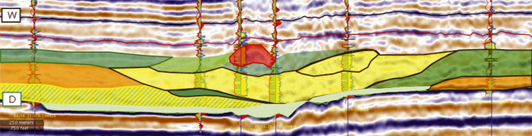
The combined interpretation of time slices and various inverted sections improve the mapping of the channel systems. An interpretation of the sections shown in figures 14 + 15 is illustrated in figure 17, with clean sand dominated bodies shown in yellow, the green color is selected for a shalier facies, orange represents sandy IHS facies, and red is for gas filled sand. This interpretation honors all well ties, however, between the wells a significant degree of freedom remains for the interpreter to analyze the data; and the given interpretation is one of many possible interpretations.

Conclusions

High quality 3 D seismic allows for reliable structural and stratigraphic mapping of the McMurray Fm. reservoir in Statoil’s Leismer license. Statistical depth conversion not only achieves high depth prognosis accuracy but also provides the tools for an estimation of the depth prediction uncertainty. A neural network analysis of multi seismic attributes enables the interpreter to map the boundaries of the reservoir and to identify thin shale layers, which could impede the SAGD process.

The resulting depth maps combined with maps for the sand shale distribution allows for good estimation of the bitumen in place and for optimizing positioning of SAGD well pairs. Also the number of delineation wells can be reduced.

Acknowledgements

I wish to thank Statoil Canada Ltd. for the permission to publish, H. Brekke for permission to include his HMI work, and the Leismer Asset team for their support compiling the publication, in particular A. Williams and R. Strobl.