Interpretation of Time-Lapse Seismic Data from a Heavy Oil Field, Alberta, Canada

Abstract

Two 3-D seismic datasets and their difference volume were interpreted and analyzed for the presence of amplitude anomalies and time delays related to the injection of steam into a shallow, heavy oil reservoir. High amplitude anomalies were observed on the monitor data in conjunction with apparent time-thickening of the reservoir interval due to a decrease in the P-wave velocity. The decrease of velocity was interpreted to be due to the increase in reservoir temperature and decrease in differential pressure created from the injection of high temperature steam into the McMurray Formation reservoir. An analysis of the amplitude anomalies yielded a spatial display of reservoir steam chamber distributions.

The attenuation of high frequencies beneath steam chambers was observed within the monitor survey, characterized by lowfrequency shadows, observable on the Devonian reflection underlying the amplitude anomalies.

Geological well log information was integrated with the geophysical observations. McMurray Formation channels sands were observed within the seismic data through the analysis of the semblance attribute, as well as within the geological data as low gamma ray values on well log cross sections. The channel sands were observed to intersect amplitude anomalies with the monitor volume. Outside of the amplitude anomalies, the channel sands were bound by muddy IHS bedding, creating baffles to steam flow.

Introduction

Time-lapse monitoring is comprised of a baseline survey, ideally recorded before the onset of production, and a monitor survey recorded after a period of oil, gas or water production (Clifford, et al., 2003; Kalantzis, 1996). The objective of timelapse seismic monitoring is to image production induced changes within the reservoir and to identify areas of bypassed reserves, or regions in which current steam injection is not optimally stimulating reserves. The analysis of monitor surveys may allow for the detection of both large and subtle changes within the reservoir (Johnston, 1997). To aid in the time-lapse interpretation, a difference volume was produced through the subtraction of the baseline data from the monitor data, producing a third dataset comprised of traces that are different between surveys. Difference volumes form the foundation for time-lapse seismic analysis, ideally integrated with reservoir characterization, geological modeling and reservoir production (Johnston, 1997).

The 4D dataset analyzed in this study is an ideal candidate for time-lapse interpretation. The baseline survey was recorded prior to production and possesses a high S:N ratio, while the monitor survey was recorded after nine years of steam injection and production. The monitor data contains steam chambers and elevated temperatures within the reservoir zone, albeit a lower S:N ratio due to noise contamination from production and surface activities. The strong contrast between the ideal baseline survey and a production influenced monitor survey has allowed for a detailed interpretation of reservoir changes due to production to be made.

However, observable time-lapse differences are a result of multiple factors, in which reservoir changes are one of many constituents. Differences in survey acquisition, processing, and near surface velocities during data acquisition can reduce the repeatability of a monitor survey, altering the phase, amplitude and static solution between surveys. The monitor survey was calibrated to match the phase, amplitude and statics to those of the baseline, effectively enhancing production- induced changes while suppressing differences created by other factors. Following calibration, the baseline, monitor, and difference volumes were interpreted for reservoir changes, identifying heated reservoir intervals and correlating these observations to well logs and production data.

Interpretation Overview

The interpretation of the 4D P-wave data was focused on production induced changes occurring within the McMurray Formation reservoir. The McMurray reservoir lies below the Clearwater C reflection (cap rock for the reservoir) and above the Devonian Carbonate reflection (Paleozoic unconformity). Time delays are observed along the Devonian reflection (monitor) due to a reduction in P-wave velocity of the heated bitumen sands in the overlying McMurray reservoir (see section 1.3, Chapter 1). These velocity anomalies, in combination with seismic attributes, reservoir isochrons, and amplitude anomalies, were that target of the P-wave 4D interpretation.

The interpretation of the time-lapse seismic did not include the data within the vicinity of the Quaternary channel. As discussed in Chapter 2 (section 2.3), the Quaternary channel infill is highly attenuative, preventing coherent imaging of the Quaternary channel boundaries and the underlying reflections (Figure 2-7, Chapter 2). Thus, all seismic underlying the Quaternary channel was considered to be low quality and unreliable data, and was not considered during the time-lapse interpretation.

Data Comparison

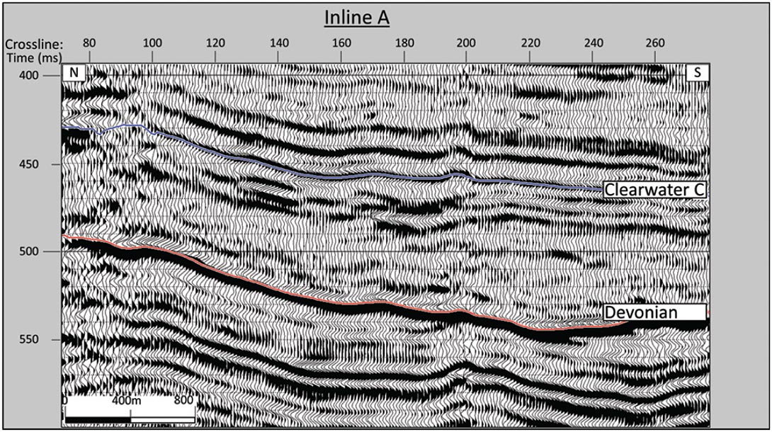
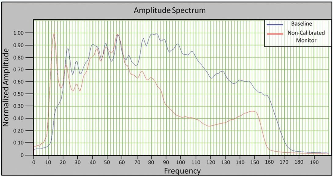
Despite the best efforts to process the data in an identical manner, there are some differences in the baseline and monitor data. Figure 1 is a comparison of the baseline and monitor data, taken from the center of the survey within an area of known steam injection. A comparison of the shallow reflections displays the large S:N and phase disparity between the baseline and monitor data. Globally, there is a phase difference of 34 degrees between the two datasets, as well as a discrepancy in the amplitudes of the higher frequencies (Figure 2). Overall, the baseline data is of higher quality than the monitor data.

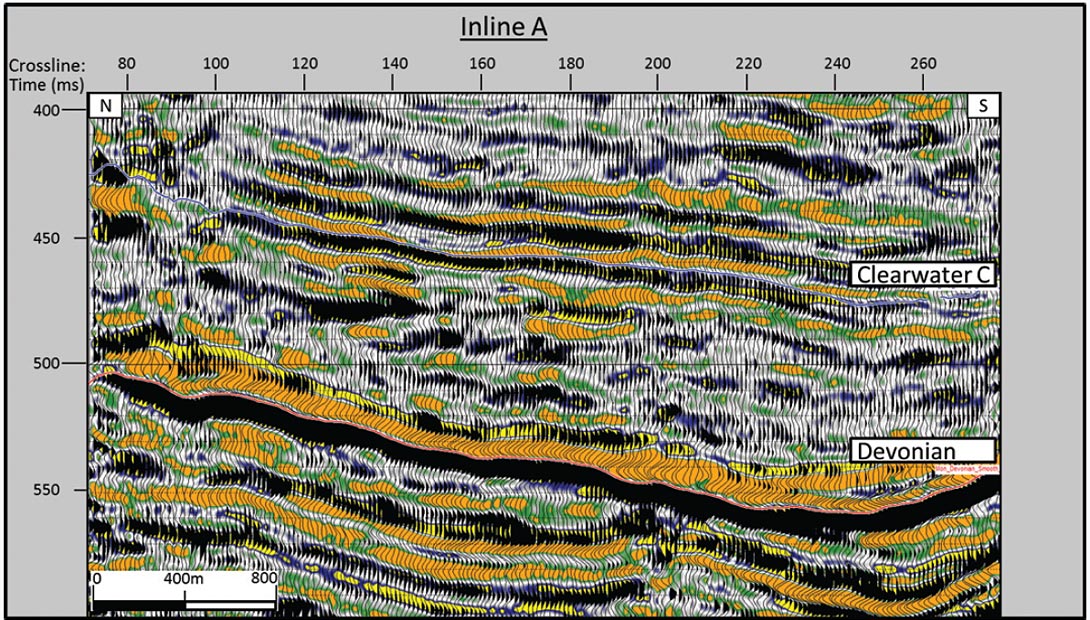
The color overlay on the monitor data is the amplitude difference between the two datasets, calculated by subtracting the baseline data from the monitor data. Positive differences are yellow and negative differences are green-orange. There are a large number of differences that due to disparity in phase, statics and amplitudes, as well as differences within the reservoir due to production. Through the calibration procedure, non-production induced differences were reduced, while steam related anomalies were preserved.

Horizon Interpretation

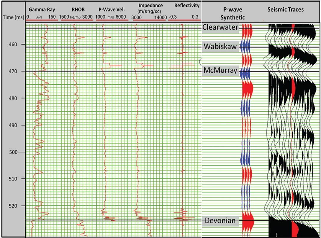
Prior to interpretation, the temporal positioning of the reservoir and reflectors of interest was determined. The main geological units of interest are represented as seismic horizons corresponding to the Devonian Carbonates of the Beaverhill Lake Group, the Clearwater B Formation, and the Clearwater C Formation (cap rock). Each horizon was identified within the seismic data through the correlation of seismic reflections with geological units, where geological well tops identified on sonic logs were related to seismic reflectors via synthetic seismograms. The synthetic seismograms were generated by the convolution of the reflectivity series with an Ormsby wavelet containing a frequency range representative of that within the data. Figure 3 is an example of a synthetic seismogram tie for well A displaying well log tops for the Devonian, and Clearwater C Formations, and their relationship to the seismic data. Following the well tie, seismic horizons were picked on the zero crossing for each reflector of interest. Horizons were initially picked on the baseline survey and noncalibrated monitor survey, and after data calibration, re-picked on the monitor survey.

Inital Interpretation

Before data calibration, a preliminary interpretation of the baseline and non-calibrated monitor survey was performed to gain an understanding of amplitude anomalies observable within the reservoir interval. The interpretation of this time-lapse dataset was focused on the McMurray Formation reservoir, lying between 450-550 ms, bound above by the Clearwater C horizon and below by the Devonian horizon.

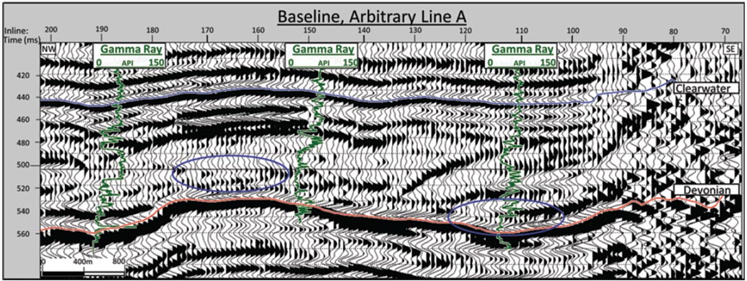
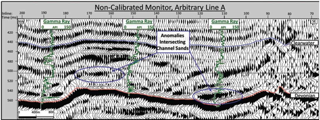
Figure 4 is a seismic cross section taken along an arbitrary line running NW to SW through both the baseline and non-calibrated monitor data, focused on the McMurray Formation reservoir. Between inlines 160 and 180, at a time of 500 – 510 ms on the monitor survey, we observe a high amplitude event which is not observed on the baseline survey. This high amplitude event coincides with a velocity pushdown along the Devonian reflection of 6 ms. Overlaying gamma ray logs onto the baseline and non-calibrated monitor data demonstrates that the high amplitude anomaly intersects a low gamma ray value, representing a channel sand within the Lower McMurray Formation. The intersection of an amplitude anomaly with reservoir channel sands is interpreted to be indicative of a steam induced anomaly.

A second high amplitude event is observed on the non-calibrated monitor data between inlines 100 and 120, at a depth of 530 – 540 ms, which is also not present on the baseline data. This event coincides with a Devonian time delay of 8ms, and intersects Lower McMurray channel sands, as indicated by the low gamma ray values on the overlain log. Again, this amplitude anomaly is interpreted to be due to steam injection.

Both of the amplitude anomalies are bounded by a mud or shaly unit, as indicated by a high gamma ray value overlying each anomaly. This muddy or shaley interval is a baffle to steam flow, preventing the steam from migrating upward in the reservoir to earlier times. The combination of channel sand with an overlying impermeable unit is representative of a flow conduit for steam within the reservoir. Injected steam will preferentially flow along the pours and permeable channel sands, migrating laterally throughout the reservoir while being bound to lower times due to the overlying baffle. This steam migration will bypass bitumen reserves in overlying channel sands, as steam cannot transfer heat through the shale/mud to the overlying channel sands.

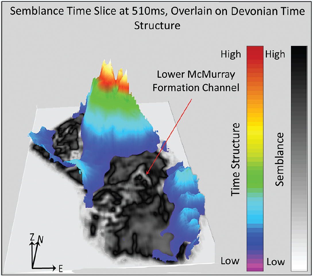
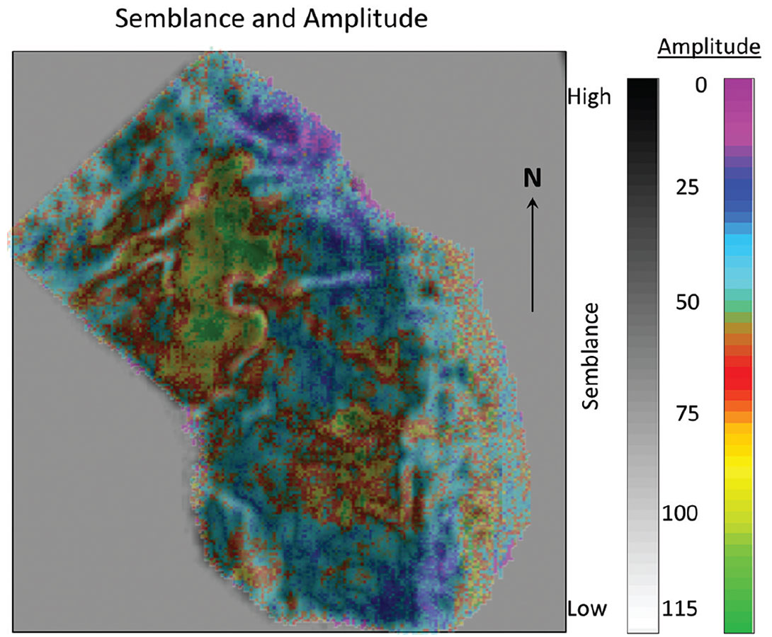
To provide further support for the presence of channels within the McMurray Formation reservoir, the baseline data was transformed into a semblance volume. Semblance is a seismic attribute, used to analyze data for changes in the seismic character, computed by comparing the amplitude of a single trace to that of an adjacent trace.

Semblance is calculated over a 3D analysis window, with a defined dip and azimuth for each point in the data volume (zero dip for a flattened volume) (Marfurt, et al., 1999; Chopra & Marfurt, 2007). Semblance is defined as the ratio of energy of the average trace to the average energy of all the traces along a specified dip, averaged over a specified analysis window. Semblance, S(t, p, q) is defined as follows:

where x_j and y_j denote the x and y distances of the jth trace from the center trace, summed over 2K + 1 samples. P and q are the apparent dips measured in milliseconds per meter and t is the time in milliseconds (Chopra & Marfurt, 2007).

Semblance values range from 0 (low) to 1 (high), where traces exhibiting a semblance of 0 have extremely different amplitudes and traces with a semblance of 1 have the same amplitudes. Effectively, semblance is a quantitative measure of the coherency of seismic data across a set of traces (Chopra & Marfurt, 2008). The semblance attribute is effective at delineating discontinuities that would cause a change in the seismic signal, such as faults or channel edges (Chopra & Marfurt, 2008). Hence, we can use the semblance analysis to identify channels within the McMurray Formation reservoir.

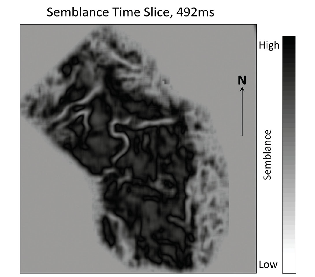
Figure 5a is a time slice through the semblance volume displaying low semblance values (white). These low semblance values are interpreted to be channels within the upper McMurray Formation reservoir.

Frequency Attenuation

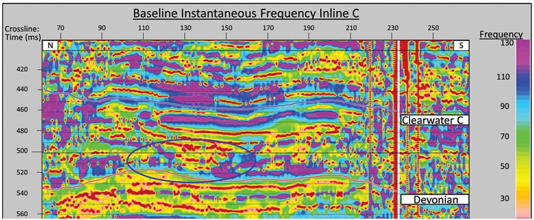
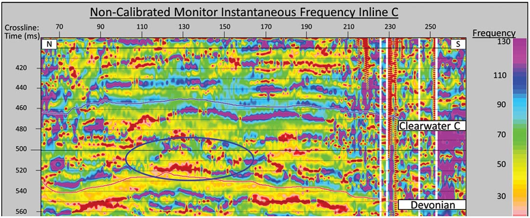
The analysis of the frequency content of the data may be indicative of reservoir steam zones. The attenuation of frequency beneath a steam induced anomaly has been discussed by Hickey, et al., (1991), Isaac (1996) and Yuwen (1998), attributing the attenuation of higher frequencies to a decrease in the viscosity of reservoir pore fluids. Velocity and viscosity are largely influenced by temperature, decreasing considerably during steam injection in conjuction with elevated reservoir temperatures above ambient values. These decreases may lead to high-frequency attenuation, where the frequency content of the reflections underlying steam zones may be characterized by low-frequency shadows (Taner, et al., 1979; Isaac, 1996; Macrides & Kanasewich, 1987). Hence, the noncalibrated monitor data was analyzed for the presence of low-frequency zones underlying observed amplitude anomalies.

Complex seismic trace analysis was employed generate an instantaneous frequency volume to aid in the investigation of low-frequency zones. Instantaneous frequency is the temporal measurement of the rate of change of the instantaneous phase, with respect to time (the time derivative of instantaneous phase (Tanner, 2002; Barnes, 2007). Instantaneous frequency is defined as (Barnes, 2007):

where θ(t) is the instantaneous phase (Barnes, 2007):

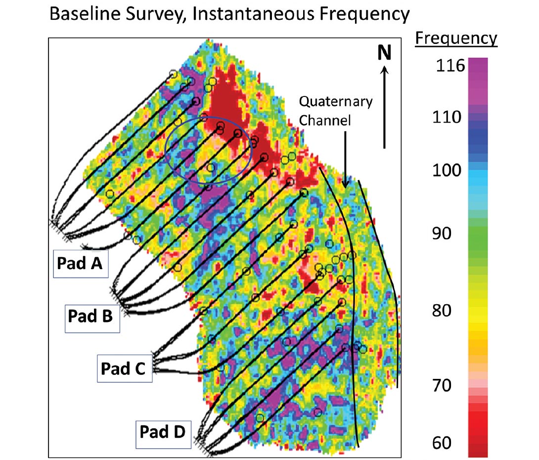
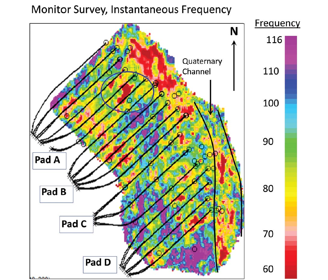
The baseline and non-calibrated monitor data were transformed to instantaneous frequency volumes using Hampson-Russell’s Pro4D software. The two amplitude anomalies observed in Figure 4 correspond with a decrease in frequency content of the events underlying each anomaly. Figure 6 is a comparison of the baseline and non-calibrated monitor instantaneous frequency volumes. There is a low frequency shadow observed at 510 ms on the monitor data between inlines 110 and 150, located on the Devonian reflection underlying the amplitude anomaly. To display the spatial distribution of the frequency attenuation, a time slice was taken through the baseline instantaneous frequency volume and the non-calibrated monitor instantaneous frequency volume (Figure 7). These time slices display the instantaneous frequency values, averaged over a 20ms window, beginning 510 ms beneath the anomaly observed between inlines 110 and 150. A comparison of the baseline and non-calibrated monitor frequency values displays the attenuation of higher frequencies on the non-calibrated monitor data, where instantaneous frequency values are significantly lower than those on the baseline data. The blue circle represents of the location of the amplitude anomaly on the time slices.

Other areas of the reservoir displayed significant frequency attenuation, as observed on the non-calibrated monitor instantaneous frequency volume time slice. Overlaying the horizontal SAGD well pairs onto the time slices displays the high correlation of horizontal wells with areas of frequency attenuation. These areas of reservoir frequency attenuation are interpreted to be representative of steam within the Lower McMurray Formation.

Data Calibration and Differencing

The time-lapse seismic surveys were loaded into Hampson- Russell Pro4D to perform reflectivity differencing of the two datasets. Prior to subtraction of the two volumes, we compared and calibrated the data to match phase, amplitude and statics between the surveys in an effort to reduce differences that are not production related. The calibration used the baseline survey as a reference, and altered the phase, statics and amplitudes of the monitor survey to match those of the baseline. The calibration procedure effectively preserved all reservoir anomalies which are related to production, while minimizing or removing all other data differences which were not related to steam injection. Figure 8 is a comparison of an inline through the monitor volume to the same inline through the baseline data.

Difference Volume

After the calibration procedure, a difference volume was created, where the baseline survey data were subtracted from the monitor survey data. This difference volume removed all repeatable traces, leaving only the difference between the two surveys. The Devonian reflection is almost completely removed from the difference section due to the matching of the Devonian event between surveys in the calibration procedure. All reflection differences overlying the Devonian event will remain, as well as any amplitude anomalies that are due to the injection of steam within the McMurray reservoir. The difference volume was flattened along the Clearwater C event to aid in interpretation. The two volumes will be referred to as (1) the difference volume and (2) the flattened difference volume throughout the remainder of this chapter.

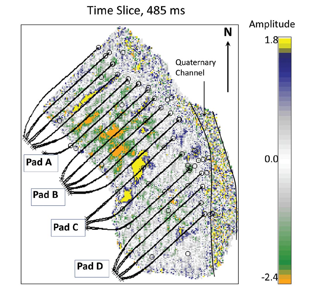
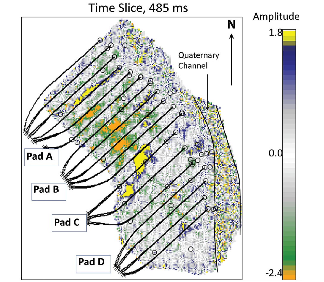
Figure 9 is an inline section through the flattened difference volume. From 470-500 ms, between cross lines 160 to 200, we observe a large amplitude anomaly, possibly representing a steam chamber. Taking a time slice though the flattened difference volume at 485 ms, and overlaying the horizontal well pairs, we observe that the amplitude anomaly corresponds with the injection wells of pads B and C (Figure 10). Thus, we interpreted this amplitude anomaly to be related to steam injection. A second anomaly is observed between cross lines 120 – 140 at a time of 460ms. Again, the time-slice displays the correlation of the anomaly with the horizontal well pairs, supporting the interpretation that the anomalies are due to steam injection into the McMurray Formation reservoir.

Observed amplitude anomalies within the difference volume appear to be located within the upper McMurray Formation, but are observed at later times on the monitor data prior to calibration. Following the global and trace-by-trace time shifts applied during calibration, the amplitude anomalies have been propagated to earlier times, and hence will be observed in the upper McMurray Formation on the difference volumes despite their original positioning within the Lower McMurray Formation on the non-calibrated monitor data.

Data Calibration Discussion

Due to the calibration procedure, time delays were removed from the Devonian reflection, shifted earlier in time through static corrections. Theses propagated time delays are observable in the cap rock region of the difference volume, where high amplitude, laterally continuous events are observed above the steam induced amplitude anomalies (Figure 9). These cap rock anomalies are created by subtracting the flat cap rock reflections of the baseline data from the reflection from the calibrated monitor survey that are no longer flat due to propagation of the time delays earlier in time. Hence, these anomalies represent heating of the reservoir, where elevated reservoir temperatures have reduced the velocity of P-waves traveling through the reservoir (Nur, 1982; Wang & Nur, 1988; Eastwood, et al., 1994). Reservoir temperature levels are elevated beyond the extent of the steam chambers, thus, time delays are observed to coincide with amplitude anomalies, but extend further than the lateral extent of the steam. Hence, anomalies in the cap rock region are more laterally continuous than the amplitude anomalies within the reservoir, and reflect heat distribution.

Time-lapse Interpretation

The time-lapse interpretation was focused on the identification of travel time shifts and amplitude anomalies within the reservoir, primarily observed within the difference volume. The observation of a significant time delay, coupled with an amplitude anomaly within the reservoir and the correlation to horizontal SAGD wells comprised the bulk of the P-wave time-lapse interpretation.

Other techniques were employed to further support the observation and interpretation of amplitude anomalies within the reservoir, including isochronal analysis, amplitude anomaly distribution mapping, an instantaneous amplitude volume, and the integration of well log data.

Isochronal Analysis

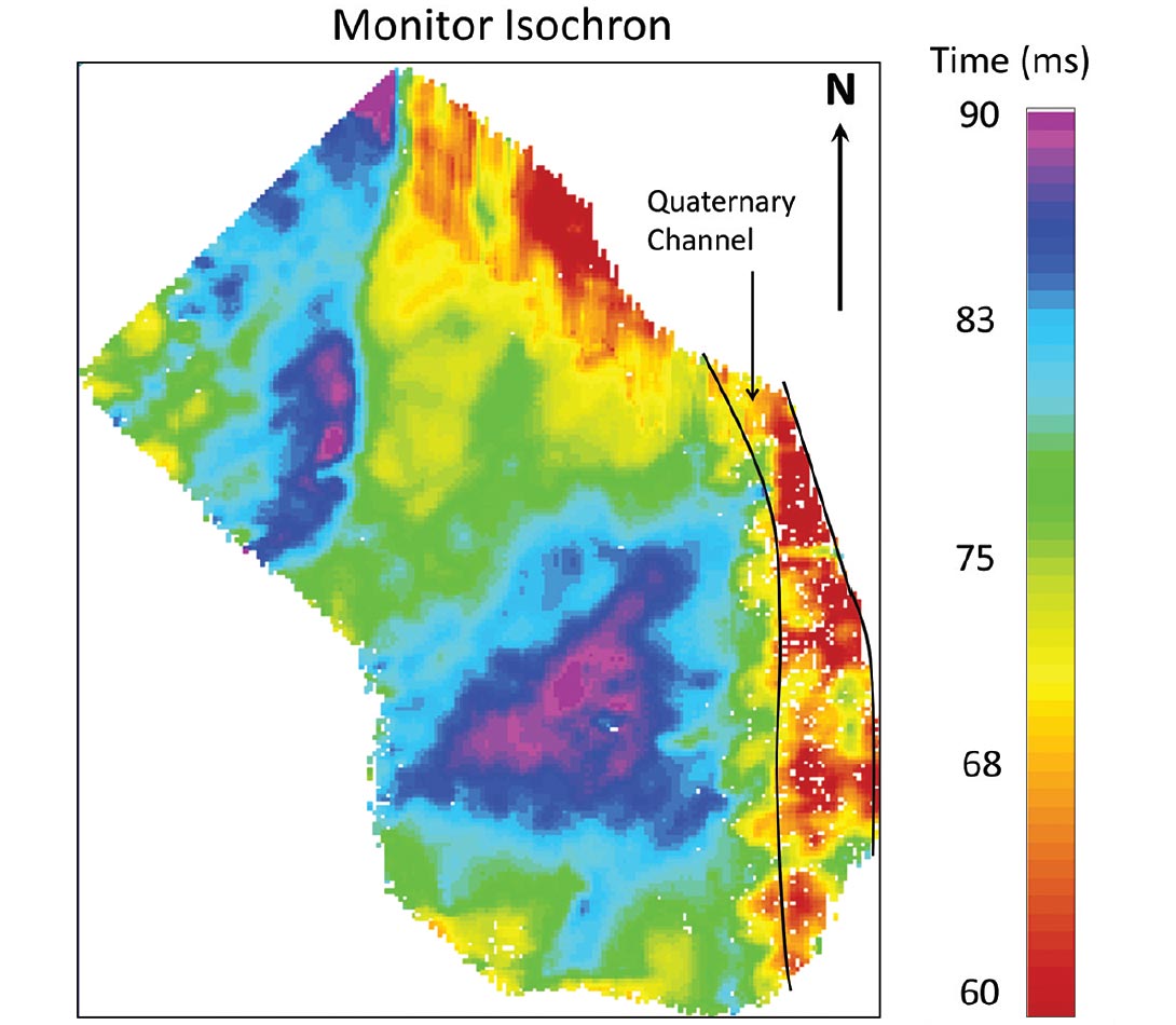
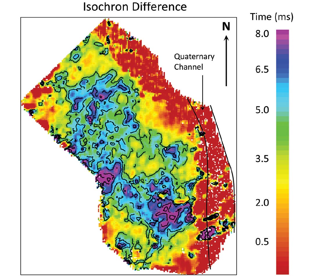
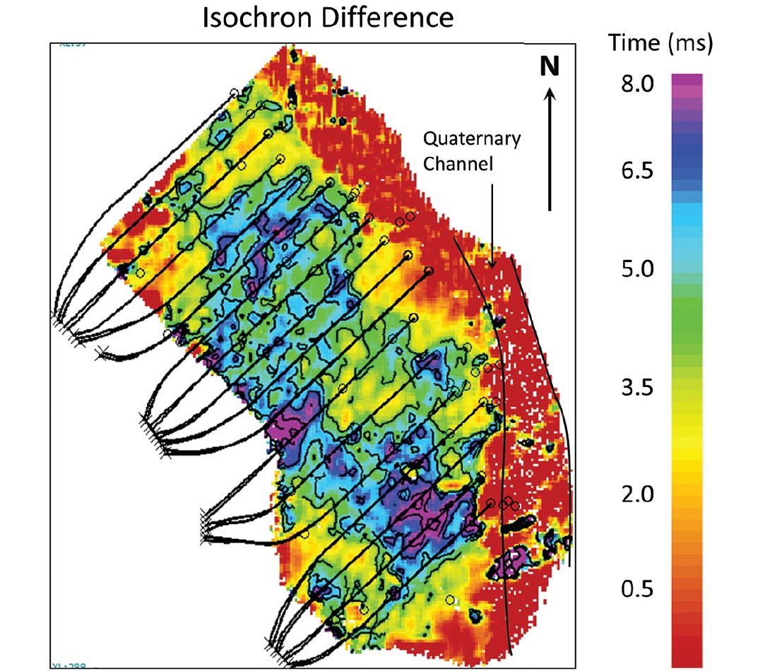
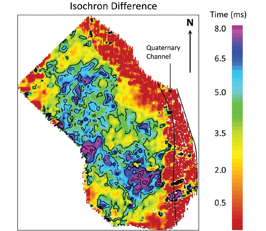
Isochronal maps display time variations between two seismic events. Effectively, they can be thought of as time thickness maps, displaying the variation in traveltime between two events (Eastwood, et al., 1994; Isaac, 1996). Isochron maps are a quick and effective technique for identifying areas of increasing or decreasing traveltime between a baseline and monitor survey. Because the reservoir thickness did not change over time, differences in isochron maps between the baseline and monitor data are representative of P-wave velocity decrease in the monitor data (Nakayama, et al., 2008). Isochrons were built over the reservoir interval, bounded by the Devonian horizon and the Clearwater C horizon on both the baseline and calibrated monitor data. Figure 11 is a comparison of the baseline and monitor isochron maps. There is significant travel time thickening in areas of steam injection, due to the traveltime delay created by the lower velocity of heated bitumen. The injection of steam into bitumen saturated reservoir reduces P-wave velocity up to 30 percent (Wang & Nur, 1988; Eastwood, 1993). A velocity reduction will create time thickening within the reservoir, represented as an increase in isochron thickness in a time-lapse sense. Taking the difference of two isochrons accentuates the time delays (Figure 12)

It is important to consider that the decrease in velocity signifies heating of the reservoir and not solely the presence of steam. The reservoir can be heated at a distance greater than that of the steam distribution. Thus, there are portions of the reservoir which do not contain steam but have elevated temperatures, creating a traveltime increase. Consequently, the isochron difference map is representative of the heat distribution and not of steam distribution.

Amplitude Anomalies

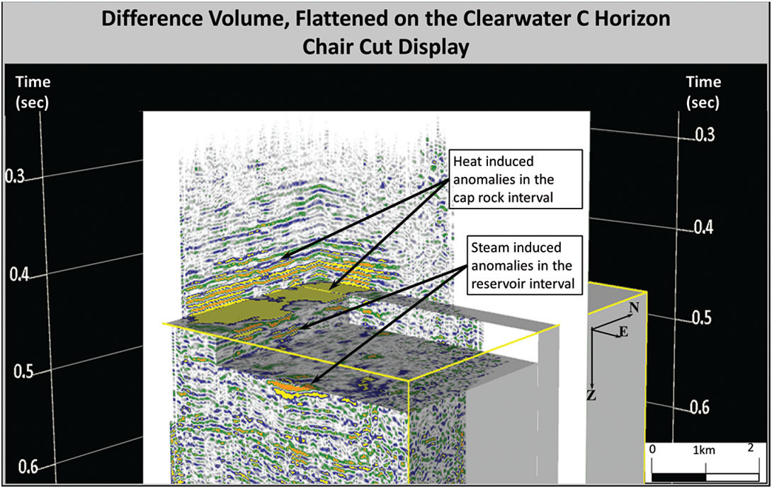
The flattened difference volume was analyzed for the presence of amplitude anomalies within the McMurray Formation reservoir. Figure 9 shows an inline though the center of the difference volume displaying two anomalies interpreted to be due to the injection of steam into the reservoir, with overlying anomalies in the cap rock due to heating induced time delays. Figure 13 is a chair cut display of the flattened difference volume, combined with an intersecting inline and crossline, displaying time delay anomalies within the cap rock interval, as well as steam amplitude anomalies within the McMurray Formation reservoir. As previously discussed, anomalies due to time delays were observed within the caprock interval, while anomalies due to steam injection were observed within the McMurray Formation reservoir.

Reservoir amplitude anomalies were observed throughout the difference volume and largely correspond with locations of horizontal wells and also with isochron time delays (Figures 9, 11). This identification procedure was employed throughout the flattened difference volume, yielding multiple observations of amplitude anomalies within the McMurray reservoir.

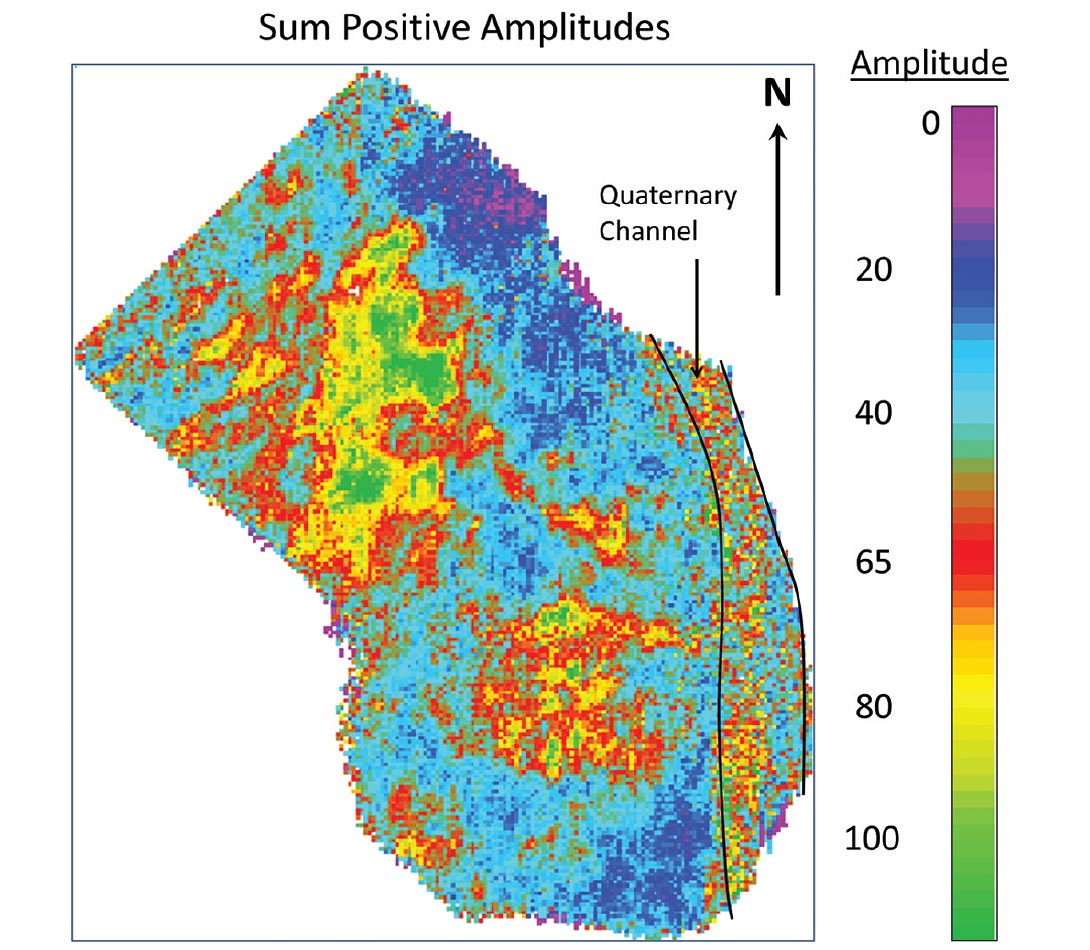
To garnish our understanding of the distribution of amplitude anomalies throughout the entire reservoir, we adopted a technique developed by McGillivray (2005) for identifying the spatial distribution of heat within a reservoir. Using the flattened difference volume, the positive amplitudes were analyzed throughout the McMurray Formation reservoir. The reservoir interval was defined as the time interval 5ms lower than the flattened Clearwater C horizon to the Devonian horizon. The addition of 5 ms to the Clearwater C horizon ensured that the calculation of the amplitude anomalies did not include the anomalies present within the cap rock interval. Amplitude values were analyzed on a slice-by-slice basis, summed and displayed in map view, yielding the total distribution of the positive amplitude anomalies within the reservoir. This technique was also applied to the largest negative amplitude anomalies. Figure 14 is a map view of the positive and negative amplitude distributions. There are two large amplitude anomalies in the study area, one in the north corresponding to pads A and B and one in the south corresponding to pads C and D. Overlaying the well pairs onto the anomaly distribution maps highlights the correspondence of well placements with amplitude anomalies.

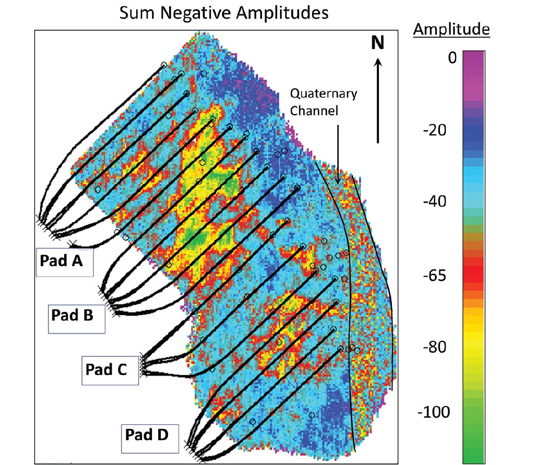
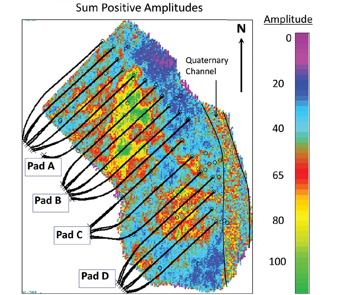
The anomalies on both the positive and negative distribution maps appear to follow the paths of the horizontal wells. From this, I interpret that the amplitude anomalies contained within the McMurray reservoir interval are likely a result of steam injection and thus are representing the reservoir heat and steam distribution in a spatial display.

The observed amplitude anomaly distributions coincide with areas of increased traveltime. Figure 15 is a comparison of the isochron difference map to the positive amplitude anomaly distribution map. A strong correlation between traveltime delays and amplitude anomalies were observed, thus supporting the interpretation that the increase in traveltime within the McMurray Formation reservoir on the monitor survey is a result of reservoir heating, creating a time delay for waves propagating through the reservoir. However, the distribution of time-delays is greater than that of the amplitude anomalies. Reservoir temperatures levels are elevated beyond the extent of a steam chamber, creating time delays that are not associated with amplitude anomalies within the McMurray Formation reservoir. Thus, the isochron distribution map is representing the distribution of heat within the McMurray Formation reservoir, while the amplitude anomaly distribution map is representative of steam-induced anomalies (the amplitude anomaly distribution maps did not include the amplitude anomalies of the cap rock region that were created from the calibration procedure).

Northern Anomaly

A further point of interest is the asymmetry of the heat distribution. Although the amplitude anomalies tend to follow the horizontal well paths, the anomaly in the north also contains a northern trend, perpendicular to well orientation. The flow pathway of the heat appears to be between injection wells, connecting the well pairs of pad B to those of pad A. Pads A and B produced approximately 3.61 million barrels of oil from February 2008 to January 2011, the latter being the time of recording of the monitor survey.

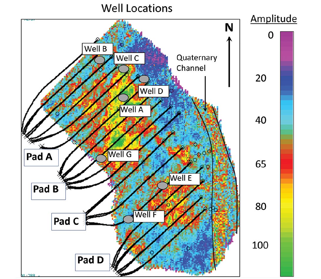
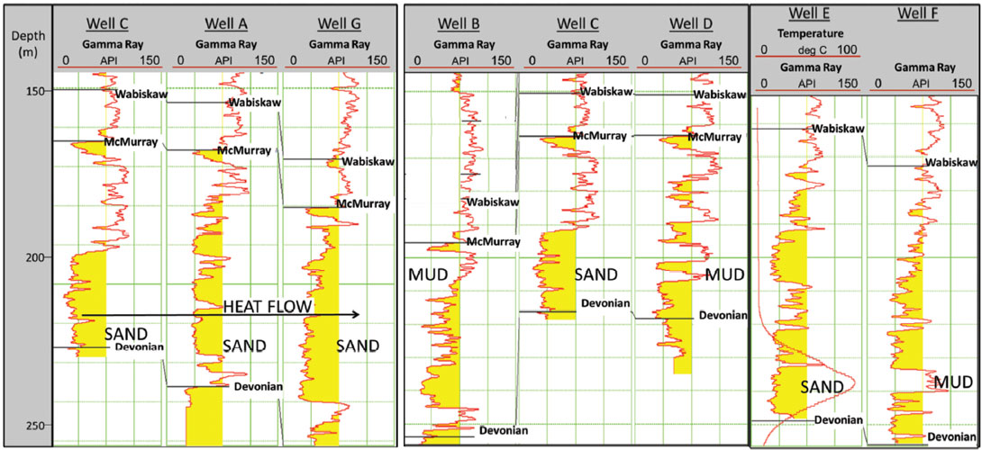
Figure 17a is a well log cross section running SW-NE along the northern amplitude anomaly. There is a very large succession of channel sands observable from the gamma ray logs, through which heat may flow from the wells of pad B and connect to the wells of pad A to the north.

The amplitude anomaly terminates along a NNE trend prior to the toe end of the wells, interpreted to indicate the intersection of a muddy or silty unit and inefficient steam distribution. An East-West cross-section along wells B, C and D displays a thick channel sand, bounded to the East and West by a large mud interval (Figure 17).

The boundaries of the amplitude anomaly correlate with the channel boundaries observed within the semblance volume (Figure 5) Figure 18 displays the positive amplitude anomaly distribution map overlain onto the semblance time slice at 492ms. The edges of the steam distribution show a strong correlation with the channel boundaries. This correlation is interpreted to representative of steam within a large sand-filled channel, which is bound to the east, west and northwest by muddy HIS bedding, restricting steam growth outside of the sand-filled channel. The semblance is displaying the edges of the sand filled channel.

Southern Anomaly

The southern anomaly is interpreted to show a more symmetrical heat distribution, flowing between the wells in pads C and D. This anomaly is more localized than its northern counterpart, where a significantly large area along the heel of pads C and D does not show any heating. Figure 17c is a well cross section through the southern anomaly. Well E intersects the horizontal wells of pad D, and displays a large succession of channel sands with an elevated reservoir temperature of 80 degrees Celsius. Well F to the west intersects the heel of the same horizontal well, outside of the heat anomaly, and displays a mud or shale unit structurally equivalent with the heated sands of well E. This mud may be a baffle to steam flow, currently preventing the heat from reaching the overlying channel sands. The reservoir temperature recorded in well E (80 deg C) is relatively low considering the long period of injection (November 2007- January 2011) and the higher temperatures observed in other temperature logs of 200 deg C and above. This low temperature suggests that there may be a nearby thief zone, which would steal injected heat and steam from the reservoir along the horizontal wells of Pad D.

Pads C produced approximately 1.68 million barrels of oil from May of 2003 through to January 2011 and pad D produced approximately 2.70 million barrels of oil from November of 2007 to January of 2011 for a total of approximately 4.38 million barrels of oil.

Discussion

Taking advantage of the strong contrast between the baseline survey and a production influenced monitor survey, a detailed interpretation of reservoir changes over time was carried out. Preliminary interpretation of the baseline and monitor survey identified seismic horizons of interest with the aid of synthetic seismograms and well ties, identifying the temporal location of the McMurray Formation reservoir.

Amplitude anomalies were observed within Lower McMurray Formation, which overlaid time delays and zones of frequency attenuation on the Devonian reflection. Lower and Upper McMurray Formation channels were identified within the data on semblance time slices.

Following the calibration, difference volumes were constructed to aid in the interpretation of observed amplitude anomalies. Amplitude anomalies were identified throughout the McMurray reservoir in conjunction with velocity anomalies within the cap rock (upward propagated from the Devonian after calibration).

McMurray reservoir isochrons were built using the baseline and calibrated monitor surveys to provide a quick view of time thickening within the reservoir. The reduction in seismic velocity of the heated bitumen created significant traveltime delays, resulting in velocity pushdowns, identifiable as travel time increases on the reservoir isochrons. Taking the difference between the two isochrons accentuated these time delays, which correlate strongly with observed amplitude anomalies.

Amplitude anomalies were projected into map view, providing an examination of steam distribution within the McMurray reservoir, which was contained within two main regions. Correlating these distribution maps with the SAGD injection and production well pairs provided strong support for the relationship of observed amplitude anomalies to steam injection. These maps provided a projected spatial distribution of steam within the McMurray reservoir, as well as some information regarding heat flow, and steam connectivity between well pairs.

The amplitude anomaly distribution maps correlated well with the isochron difference map. However, difference between the amplitude anomaly maps and the isochron difference maps were observed, as displayed in Figure 15. It was interpreted that the isochron difference map is representing the distribution of heat induced time delays within the McMurray Formation reservoir, while the amplitude anomaly distribution map is representing the distribution of steam anomalies within the McMurray Formation reservoir.

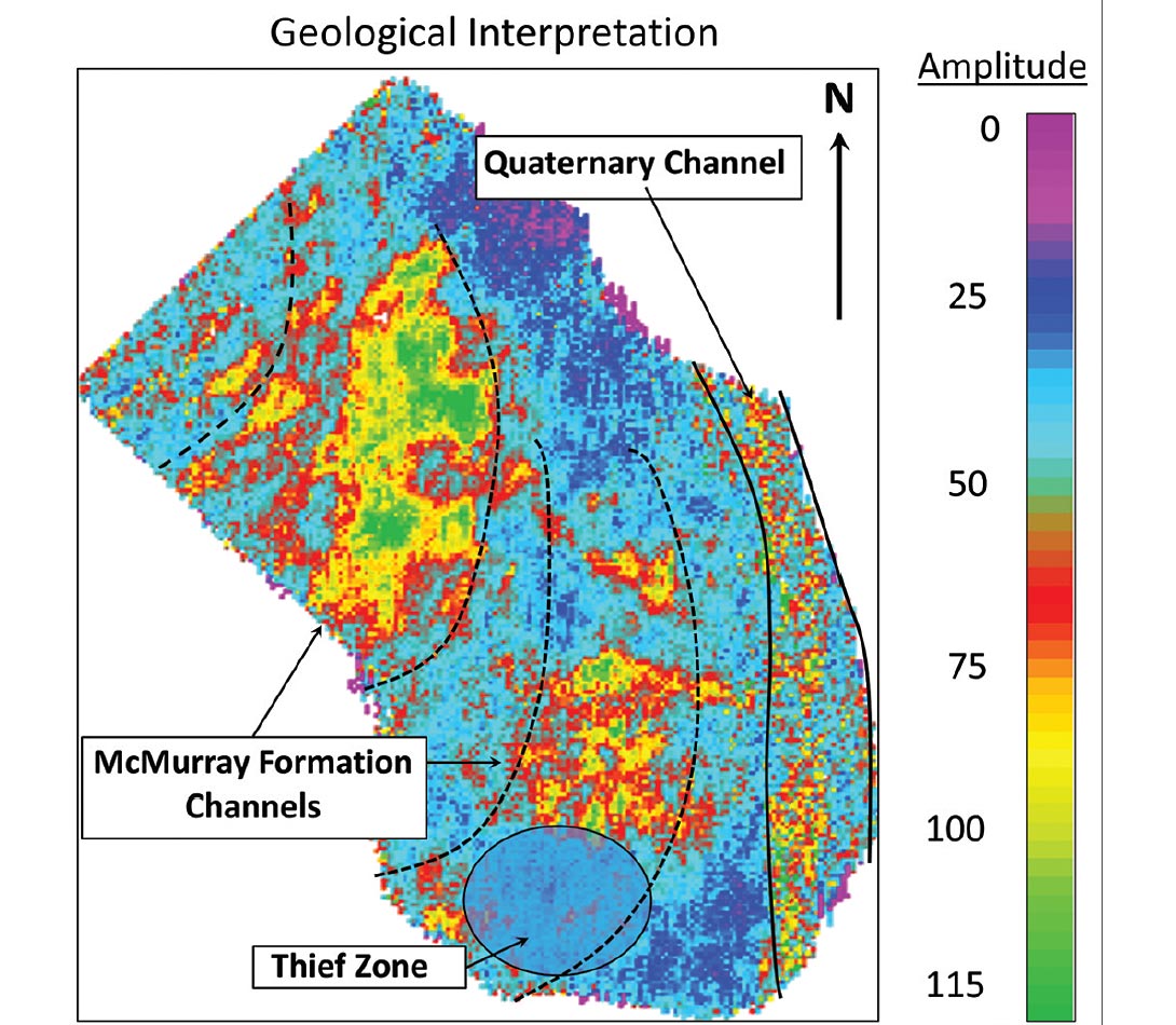
Integrating the geological interpretations provided from the well log cross sections to the geophysical observations, we interpret that the majority of the heat anomalies are located dominantly within two large McMurray channels which host the bulk of the McMurray sand (Figure 19). These two large channels trend towards the northeast, and are each comprised of a succession of smaller channels cross cutting one another. The southwest end of the southern may contain a thief zone, probably water saturated McMurray Formation sands. This interpretation was further supported by combining the amplitude anomaly distribution map with semblance time slices. The northern anomaly was observed to coincide with Lower McMurray Formation channels, where the distribution of steam appeared to be bound by the edge of a mud-filled channel contained within the larger McMurray Formation channel feature.

The area outside of the two large McMurray Formation channels was interpreted to be dominantly mud and shale, with interspersed sand. These muds and shales create baffles to steam flow, preventing heat flow and thus bypassing sand units not contained within the two large channels.

Through each of the interpretation techniques employed, a detailed distribution of steam anomalies and time-delays were presented in a spatial display. The integration of geological well logs, and the co-integration of interpretation techniques (e.g. semblance time slices with amplitude anomaly distribution maps) provided robust interpretations for the distribution of steam anomalies. The anomalies were observed to be located within large channel features of the McMurray Formation, bound by muddy IHS and restricted in some regions by thief zones. Overall, the majority of the steam was observed within two large McMurray Formation channels, comprised of an amalgamation of smaller channel features.

Acknowledgements

Thanks to my supervisor, Dr. Don Lawton for his support and advisory. Thank you to the CREWES sponsors for sponsoring this work, as well as the CREWES students, faculty and staff. Thank you to the industry donor of the data, as well as to Helen Isaac for her help processing the data.