Summary
A system for automatic, high density migration velocity estimation and imaging has been developed. The automatic migration velocity determination utilizes a set of objective norms which measure the quality of the migration as a function of velocity. Both the migrated gathers and the migrated image cube are used to calculate these objective norms. Determining the migration velocity which optimizes these objective measures is done automatically and densely.
Expectations are that the high density of the migration velocity analysis (temporal and spatial), coupled with the fidelity of the velocity determination, would also impact the initial interval velocity calculation. Utilizing the information from both the time migrated image and the imaging velocity, we show that robust initial interval velocity models are constructed and that these are applicable for curved ray and turning wave imaging (in time migration), improved amplitude corrections for AVO analysis, intrinsic VTI anisotropy estimation, 4D interval velocity differences, initial depth imaging, etc. This is explored with synthetic and real data examples, and empirical trials with a range of applications dependent on an interval velocity model.
Introduction
The economics of expanding seismic surveys has reawakened interest in automatic velocity estimation methods. At the same time, the value of high quality, high density imaging velocity analysis has been documented for nearly all aspects of post-imaging interpretation and analysis, including basic structural and stratigraphic interpretation, AVO, overpressure analysis, 4D work, and others.
To reliably and repeatably satisfy the above velocity determination needs, a data driven automatic approach was developed (Stinson et al., 2004). The velocity determination quantifies the efficacy of the prestack imaging as a function of migration velocity, through objective measures derived from both the image gathers and the image cube. The automatic iterative optimization of these objective measures to determine migration velocity has proven to be robust, repeatable, and convergent.
The objective data-driven nature of the velocity determination, the optimization approach, and the high density (in space and time) all lead to an improved time migration image and velocity field.
Automatic Time Imaging and Velocity Determination: Methodology
In the determination of velocities for imaging, the measure of success should not be a subjective issue. Any attempt to optimize the imaging results requires an objective means to quantify the current “quality” of the image and imaging velocities, and to define an update vector indicating the direction that will give improvement. This also leads naturally to automation of the optimization process.
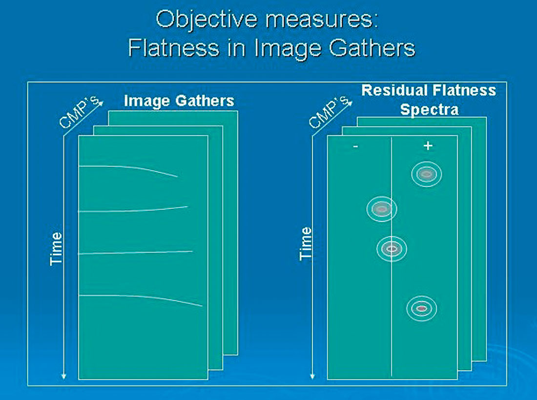
(a) Flatness of Image Gathers
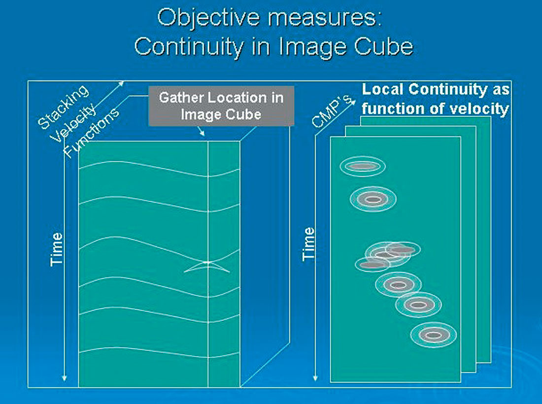
(b) Local Continuity on Image Cube
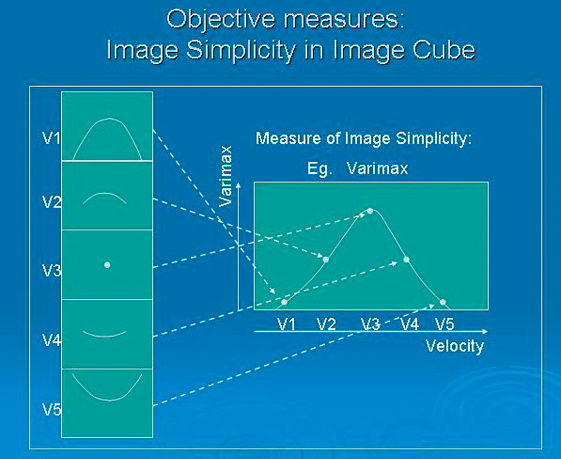
(c) Image Simplicity on Image Cube
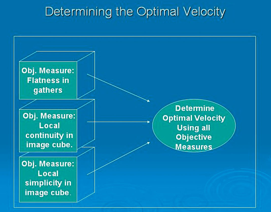
(d) Determination of Optimal Velocity
For the Automatic Imaging, a number of objective functions can be utilized that measure different aspects of the fidelity of the migration as a function of the migration velocity. For example:
- Flatness of events in migrated image gathers (see Figure
- Local continuity of events on migrated image cubes/sections (see Figure 1b).
- Simplicity or inverse entropy of events on migrated image cubes/sections (see Figure 1c).
The total objective function optimized in the automatic inversion to determine migration velocity can be a weighted combination of the individual objective measures:

| Where: | Φ 1 | measures flatness in the migrate image gathers |
| Φ2 | measures local continuity on the migrated image | |
| Φ3 | measures local simplicity on the migrated image |
For reference to conventional velocity analysis, semblance is often used to measure the flatness of events in a similar manner to Φ1. Also, constant velocity stacks are routinely visually analyzed to pick velocities on the basis of best event continuity, which is conceptually similar to what is done with Φ2 mathematically.
The weights, wi , are CMP and time dependent, and are determined by the sensitivity and robustness of the measures for different data conditions. For example, in areas of low fold or poor offset distribution (such as is often found on the edges of the survey, or at shallow times), Φ1 (flatness in gathers) is generally a poorer measure than Φ2 (local continuity in image). Similarly, at deeper times, Φ3 (local simplicity in image) is often a better measure than both Φ1 and Φ2.
In addition, issues such as local velocity continuity (in time and space), avoidance of multiples or other unwanted events, minimization of velocity variability, interval velocity checks, etc., are all handled at this velocity determination step (see Figure 1d).
Automatic Time Migration and Velocity Determination: Convergence and Repeatability
In any non-linear problem attempting to find a solution through iterative optimization, the danger of either non-convergence or convergence to local minima/maxima are present. As time migration embodies many approximations (velocity presumed to be locally invariant, primary reflections only, no converted modes or refracted waves, etc.) it is not possible to easily assess non-uniqueness or convergence except through systematic empirical trials with synthetic and real data.
Convergence
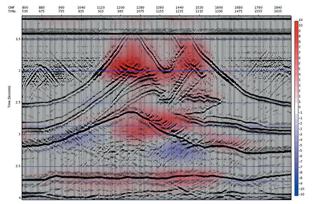
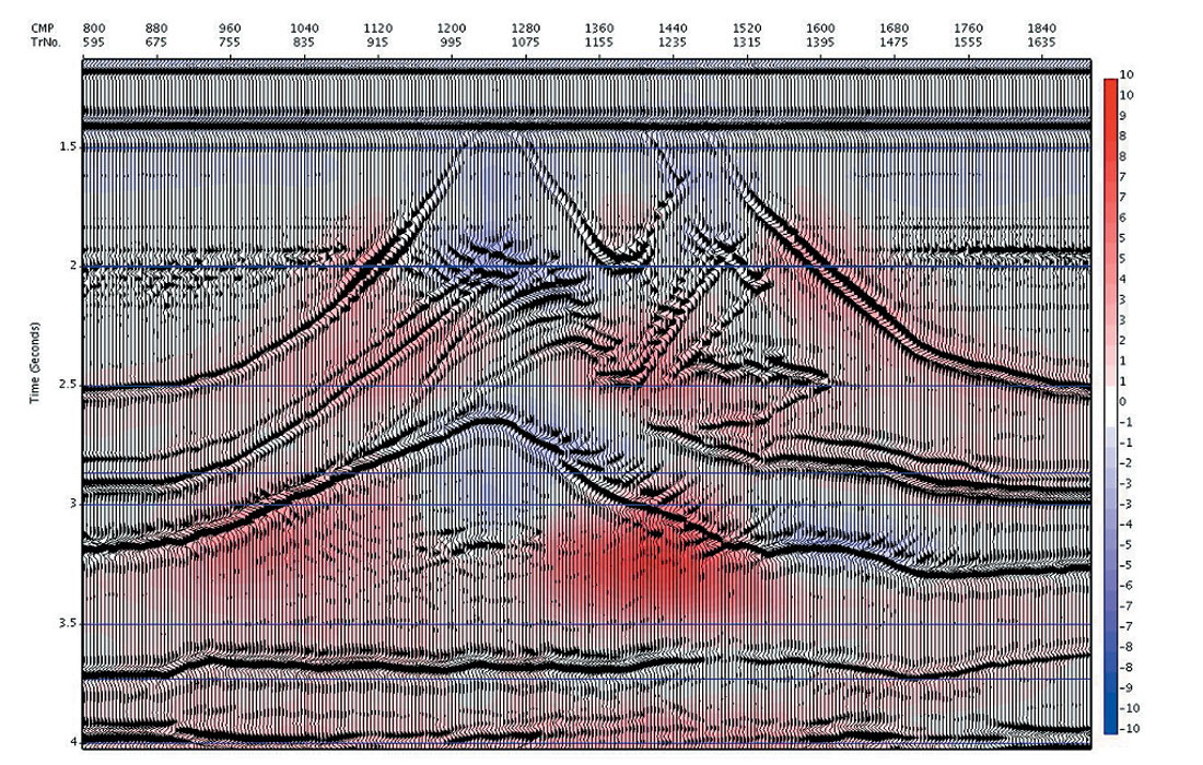
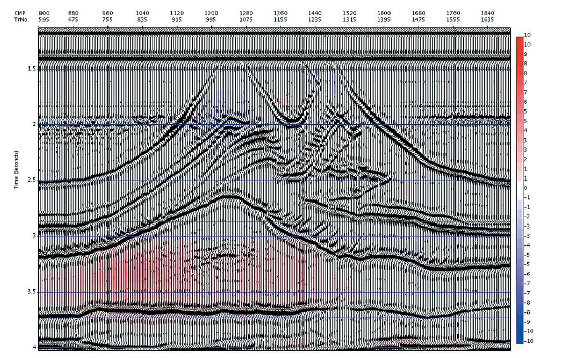
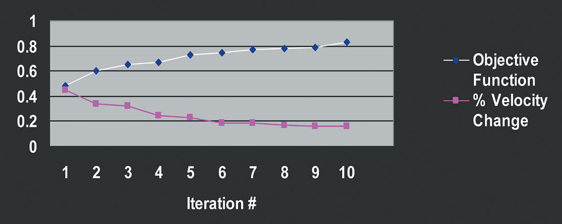
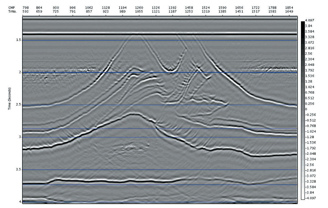
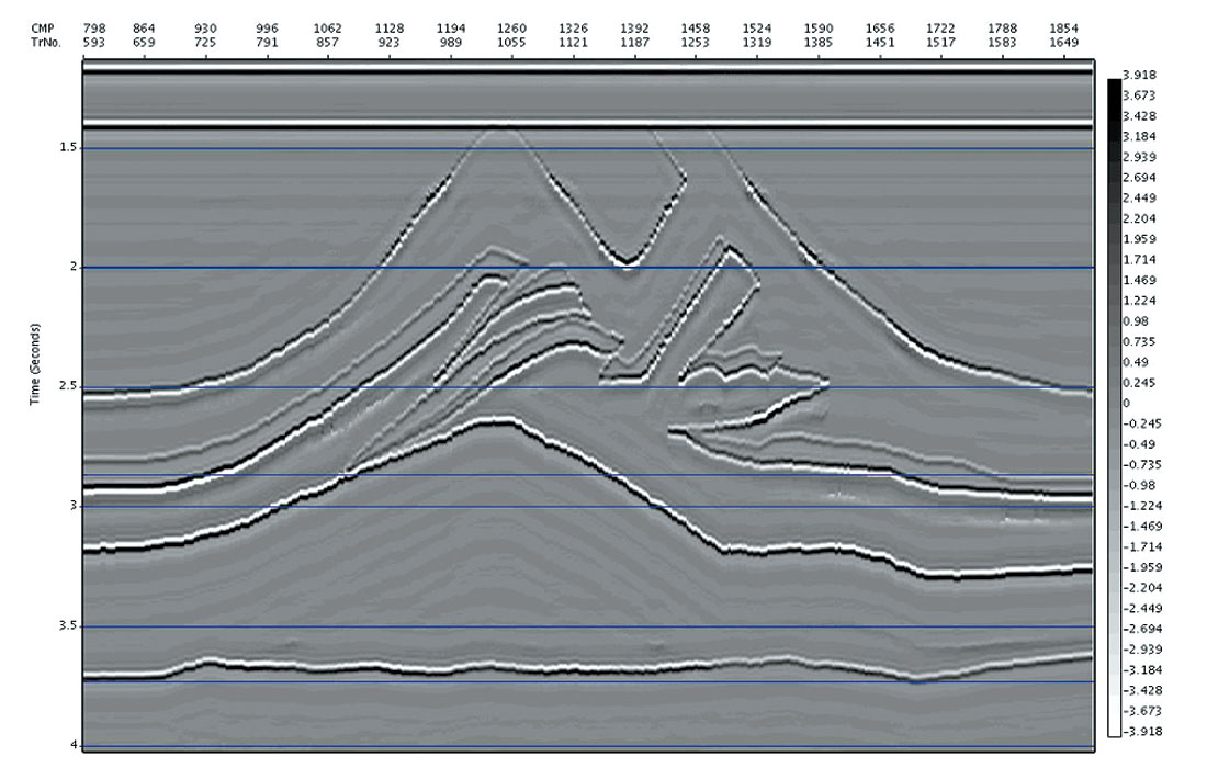
Numerous trials have shown the iterative objective optimization developed for automatic time migration to be generally convergent after 10-15 iterations from a reasonable starting model (for example, the DMO velocity). An example showing sampled iterations from a typical iterative sequence for a synthetic 2D overthrust data set is shown in Figures 2a – 2d. In each figure, the latest iteration’s migrated image is shown, with the % difference in velocity between the current and previous iteration overlain in colour. It is seen that the images gain focus rapidly in the first few iterations, and then the changes diminish, with little obvious change happening after about iteration 5. Similarly, the velocity changes are initially quite large, diminish quickly, and then after about iteration 5 are very small. We have calculated the total local simplicity using Varimax to quantify objectively our general observations, and plotted this along with the % velocity changes as a function of iteration number in Figure 3. The monotonic increase in the objective function and the monotonic decrease in the velocity differences are noted. After about iteration 5 the curves flatten out as the iteration to iteration changes approach zero, indicating convergence to a final solution.
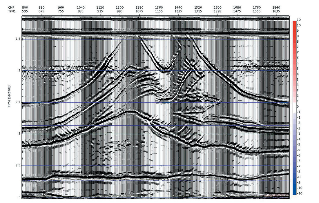
In Figure 4a and 4b we compare the image at iteration 8 with the model reflectivity (compressed vertically to time). (Note that post migration time is measured along the image ray, whereas the model reflectivity time is measured along the vertical, so there may be positioning errors of events underneath areas of lateral velocity heterogeneity).
Repeatability
In our empirical testing of the uniqueness of the solutions, and susceptibility to converge to local rather than a global optimum, practical trials were performed in which the initial velocity was varied (within reasonable general velocity limits). In all such cases the final velocity models and respective images were very close in both appearance and absolute measures despite differing starting models, except for areas of the data where the fold or offset distribution was so poor that the data did not limit velocity possibilities.
 >
>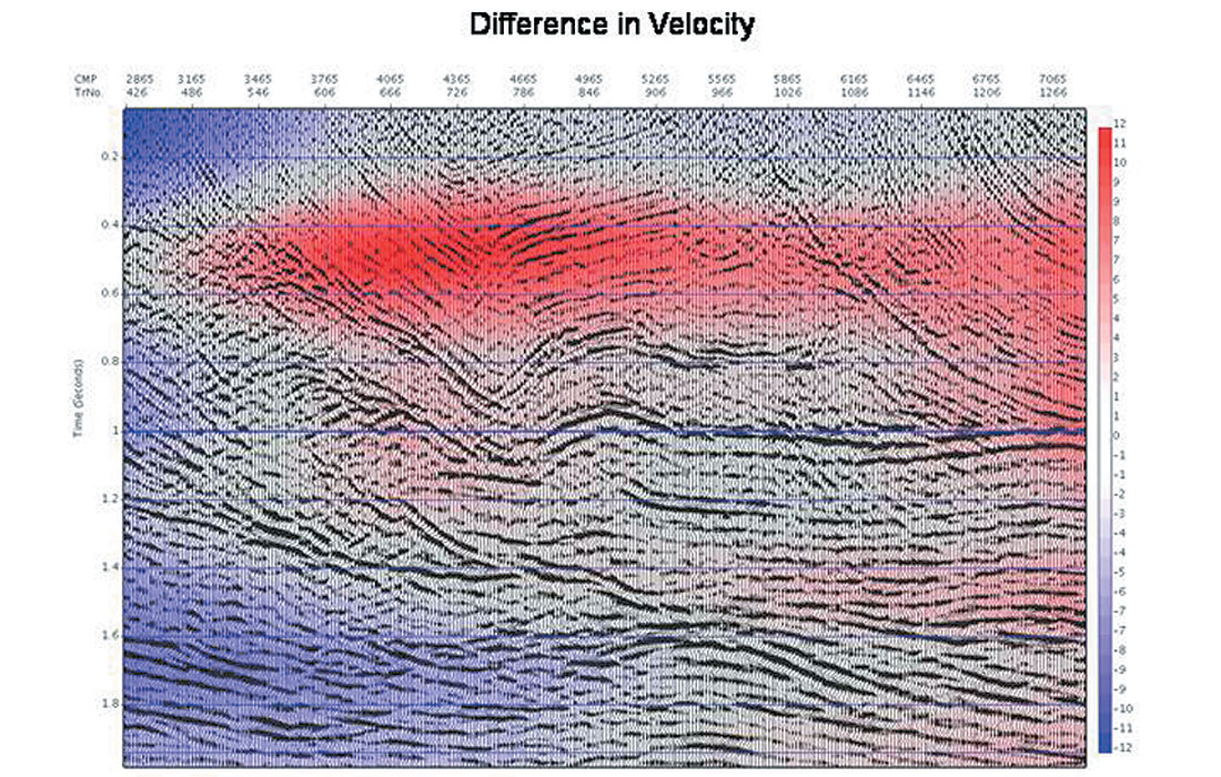
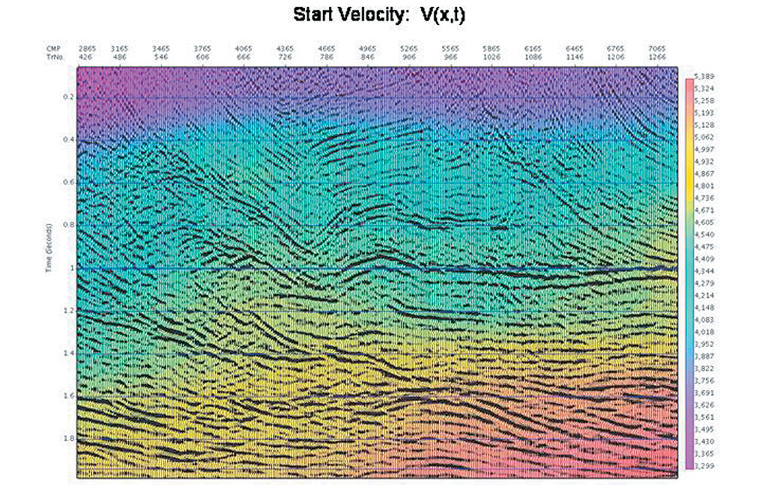
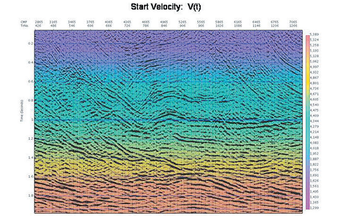
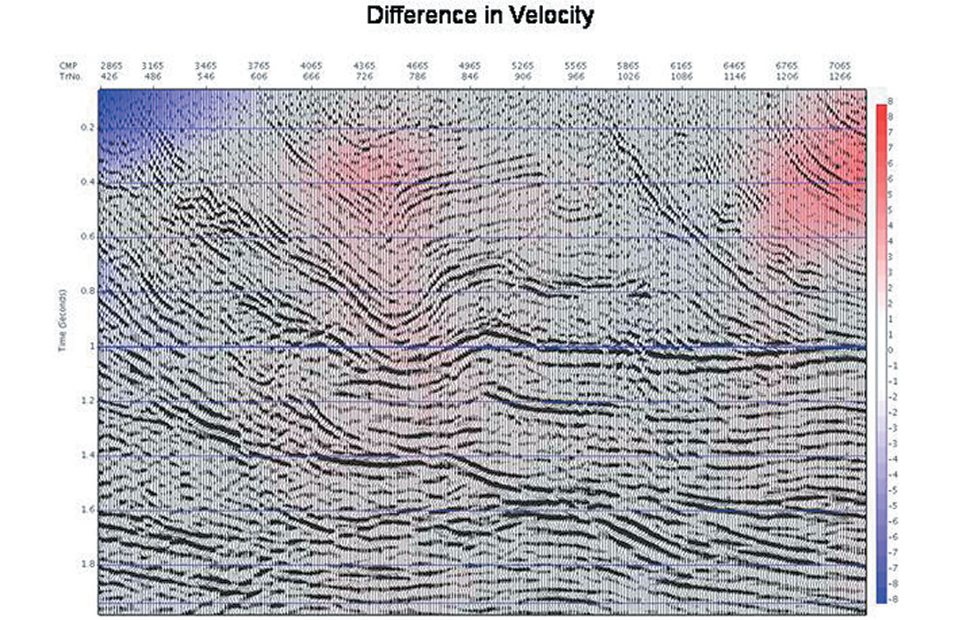
As an example of these trials, shown below is the Benjamin data set (Mewhort and Stork, 1995). In Figure 5a and 5b we show the time migrated images using two different initial velocity models (the time migration velocities are overlain in colour). The actual % velocity difference is shown as well in Figure 5c, and contains differences as large as 12%.
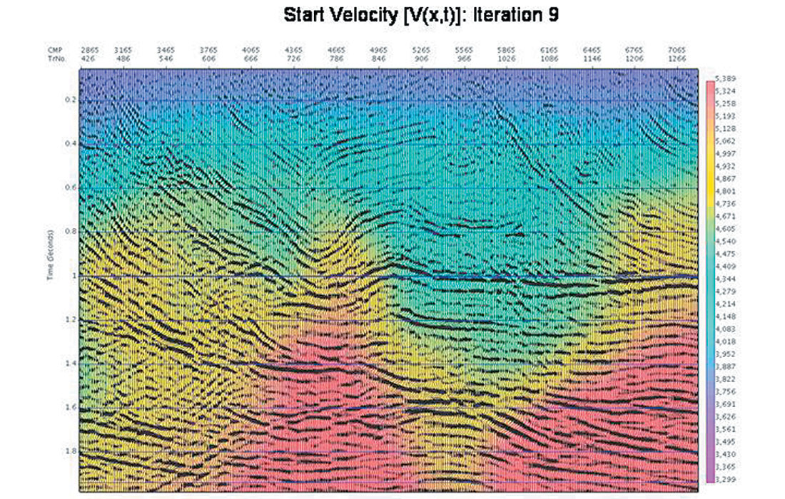
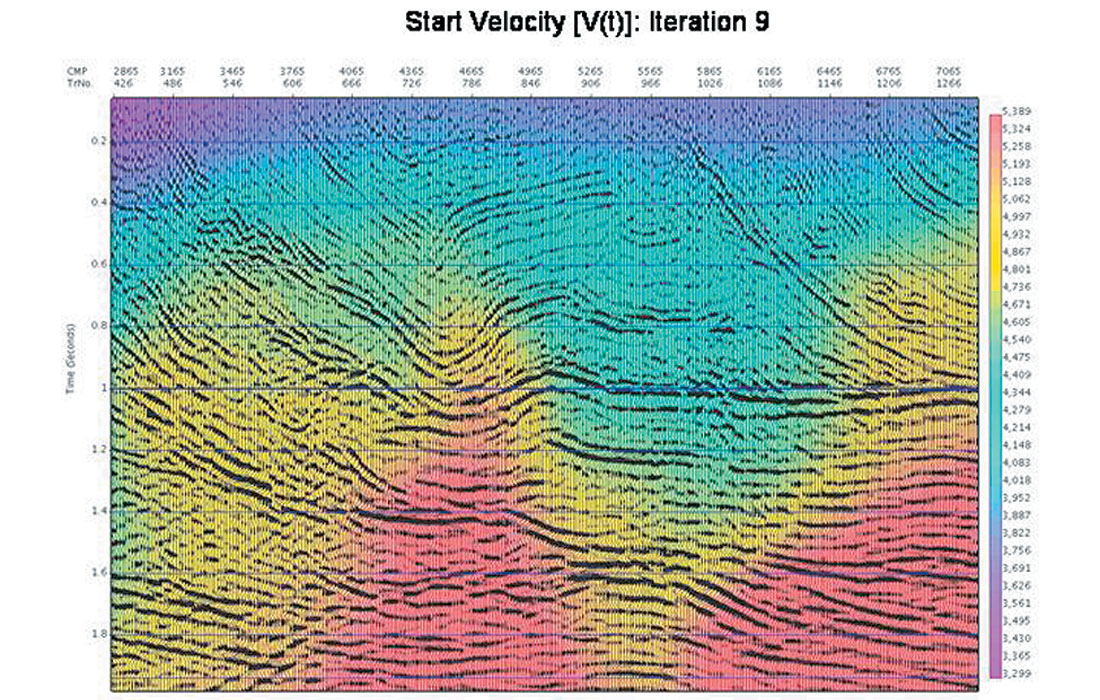
After 9 iterations of the automatic velocity determination, the time migrated images (Figure 6a and 6b, with migration velocities overlain) were both visually very similar. The actual % velocity differences (Figure 6c) confirm this, with differences on the order of a percent or less everywhere except in the shallow corners where the fold tapers to zero due to the roll on/off of shooting. The improvement of the images (from either starting velocity) is also to be noted.
Automatic Time Migration and Velocity Determination: 3D Examples
SEG/EAGE Salt Model Synthetic
The 3D Salt Model synthetic data set produced jointly by the SEG and EAGE has been widely used in publications as a test data set for time and depth migration algorithms, with the velocity presumed to be already known (that is, the given exact velocity is used). However, it is much rarer to see it used for the problem of actually determining the migration velocity model. In this test of the Automatic Imaging, we start with no knowledge of the velocity model, and proceed to automatically determine the time migration velocity and migrated image. Although the entire cube was imaged, and there are many areas of interest (with respect to imaging and velocity determination) in the cube, we only show a representative time slice and a cross line that is compared to the same cross line from the true reflectivity cube (compressed to vertical time).
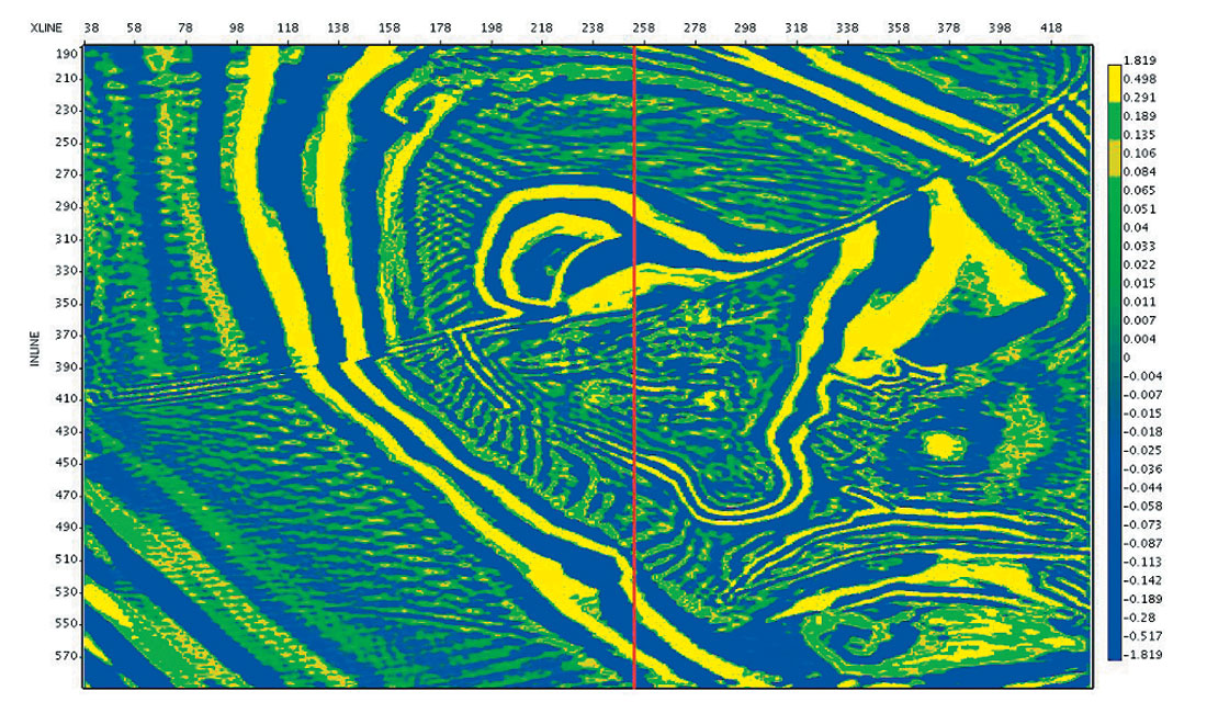
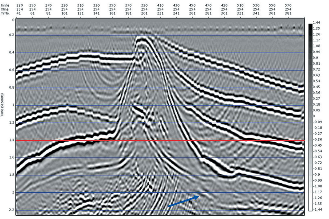
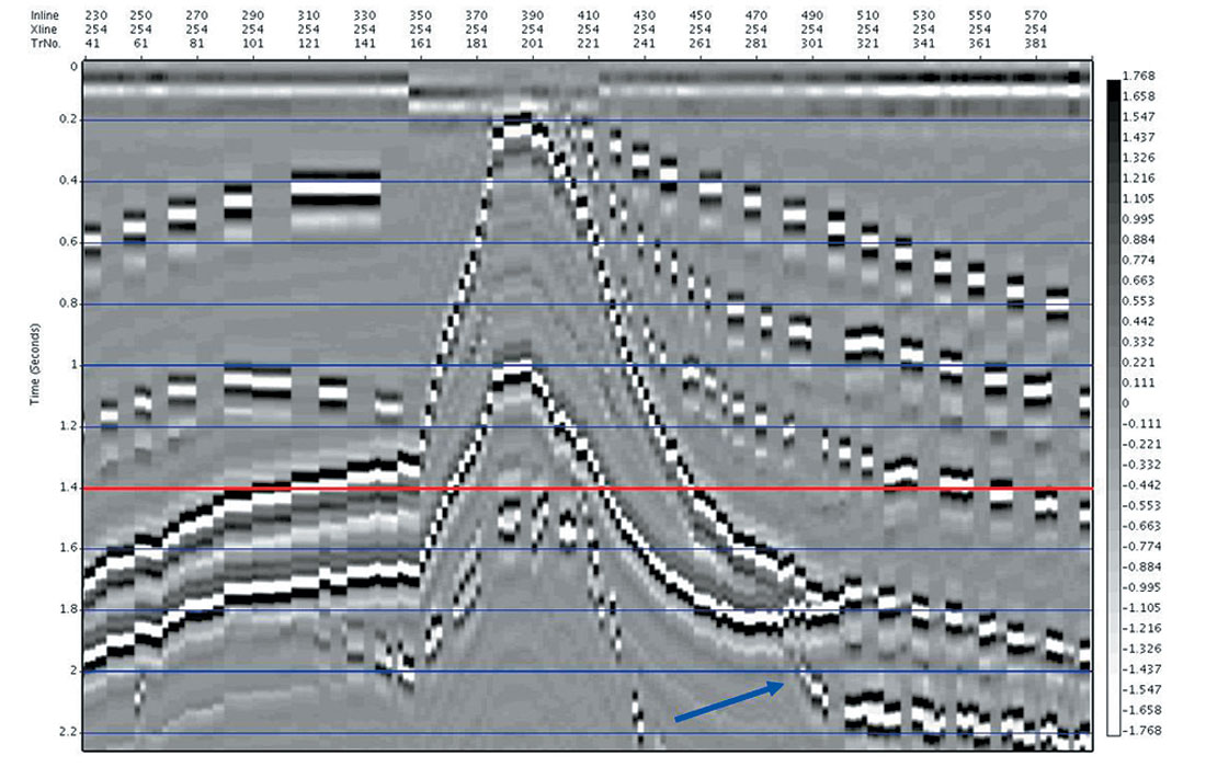
In Figure 7a, we show the time slice at 1.4 sec from the Automatic Imaging cube. Marked on the time slice with a red line is the location of cross line 254. In Figure 7b, we have cross line 254 from the Automatic Imaging cube, and for comparison in Figure 7c, we have the same cross line from the true reflectivity cube (compressed to vertical time). Note that events in the time migrated cube are imaged along the image ray, so that events may be mispositioned compared to the true reflectivity compressed to time, especially under areas of velocity complexity (such as the salt). An example of this is the subsalt reflector on the right hand side of Figure 7b, which has been imaged well, but is mispositioned due to the bending of the image ray (see blue arrows).
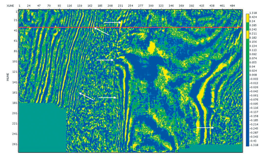
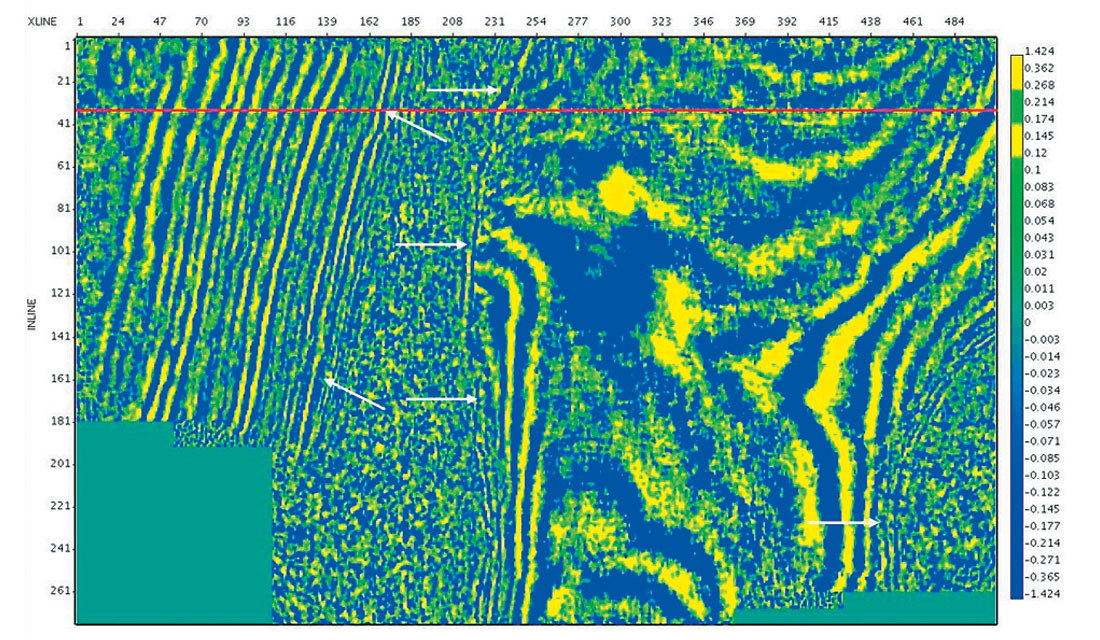
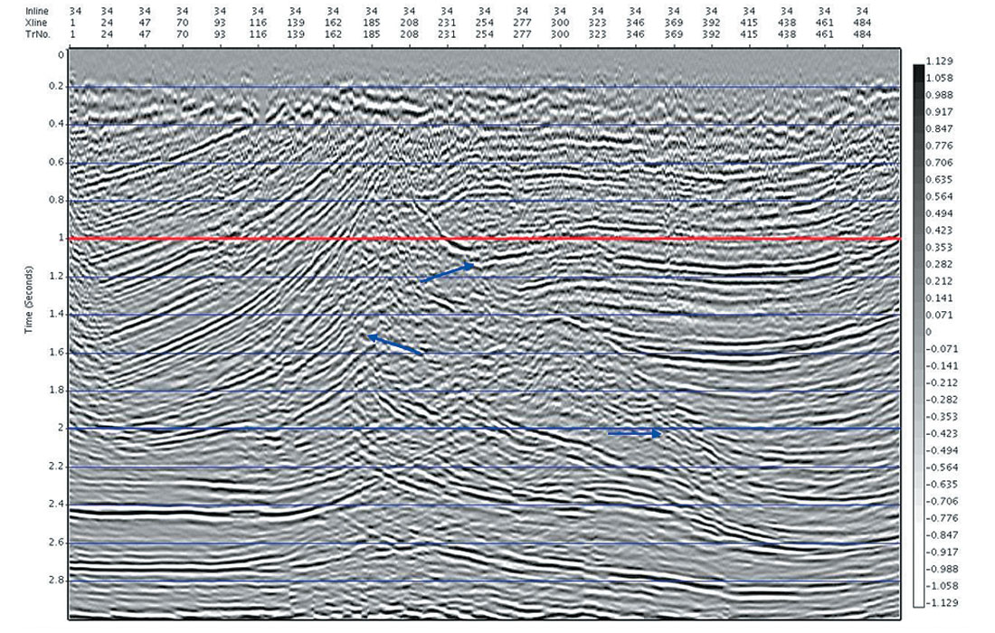
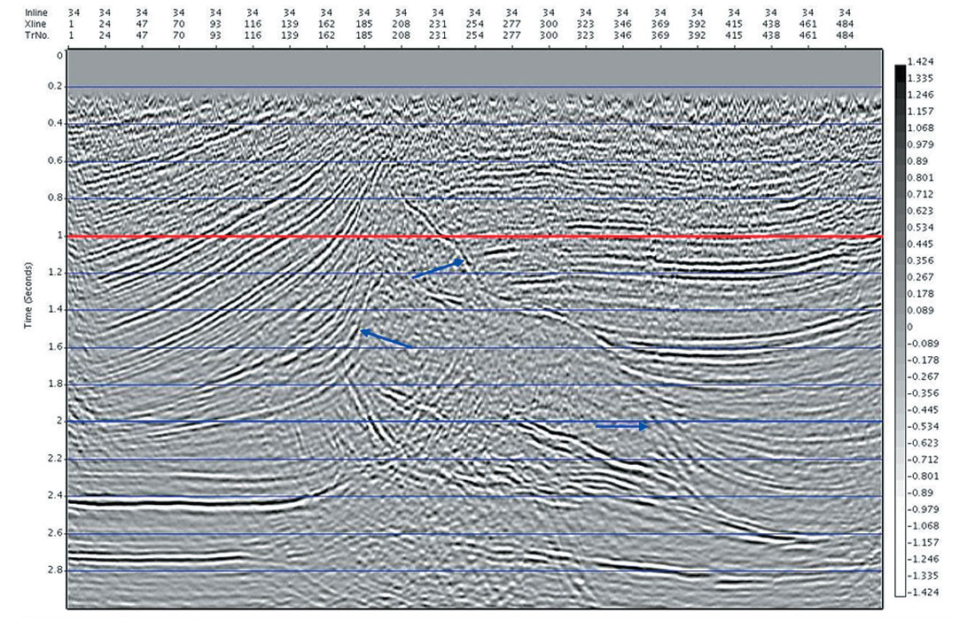
3D Examples: Land 3D – Manual vs Automatic
In the following land 3D example, migration velocities and final prestack time migrated images were determined independently by another group, allowing comparison to the results from the Automatic Imaging approach. Shown in Figures 8a – 8d are comparisons of the Manual and Automatic results for a time slice at 1.0 sec, and inline 34. Although it is obvious that the manual work could have been more complete, the following comparisons exemplify data for which automatic velocity determination is a necessity. It is clear that the dense nature and consistency of machine controlled velocity estimation is of utmost importance where imaging velocities must change quickly, such as is the case on the flanks of salt. The white arrows on the figures point out areas where the density, consistency and veracity of the Automatic velocities has resulted in superior imaging of the salt flanks.
“Soft Depth” and Depth Applications: Constructing and Using the Interval Velocity Model
Automatic Imaging determines optimal time migration velocities from time migrated images and gathers that maximize the objective quality measures as per Equation 1.
With the fidelity obtained from objective optimization, and the dense velocity field made possible by an automatic approach, an interval velocity model derived from the time migration velocity and image also has increased veracity.
We distinguish two types of applications for which we use interval velocity models:
- Soft Depth: applications that leave the output in the time domain, but for which we use information derived from the interval velocity model. These include:
- amplitude restoration migration for AVO analysis
- curved ray and turning ray migration
- Depth: depth migration
For “Soft Depth” applications, the interval velocity is simply calculated by a standard Dix methodology.
For Depth migration, our interval velocity model is constructed by a constrained Dix inversion (solved using Linear Programming), in which horizon constraints are imposed on the solution. Note that this is only an initial guess model, and so no effort is made to migrate the velocity model from the image ray to the vertical coordinate.
Examples of the two interval velocity construction approaches are seen in the following examples.
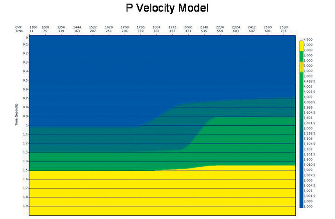
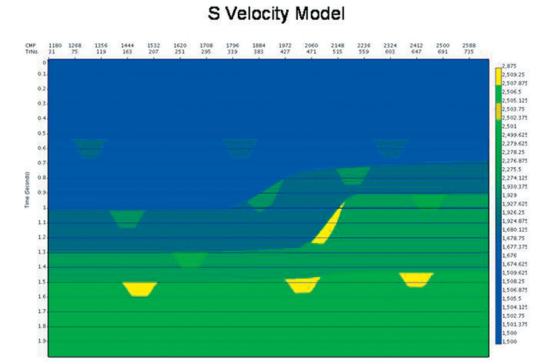
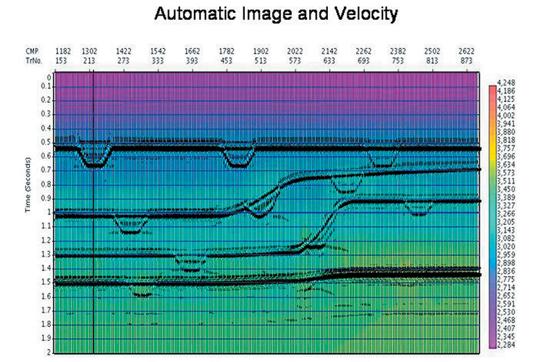
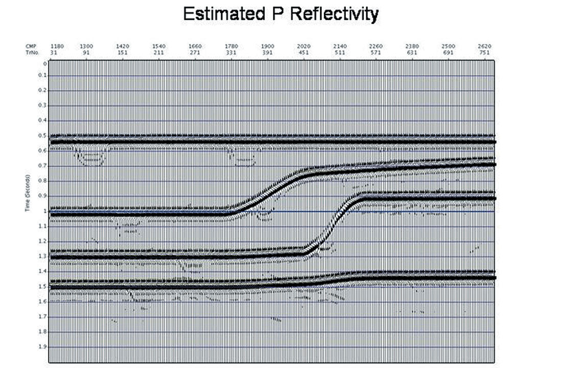
Soft Depth: AVO
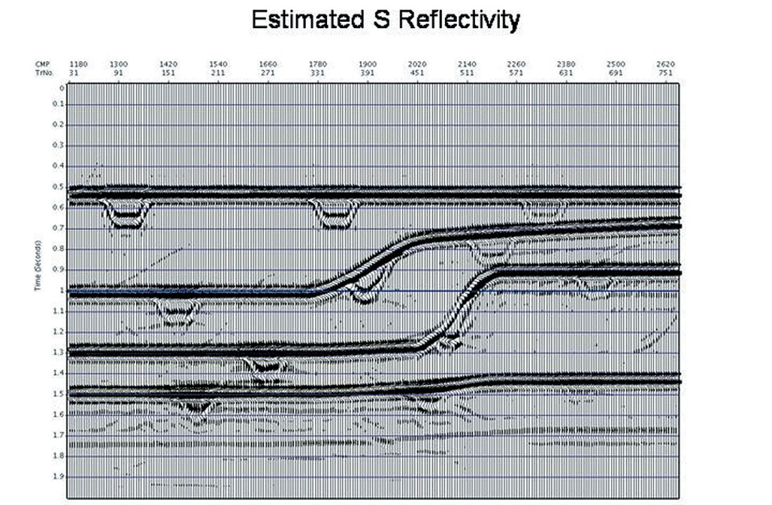
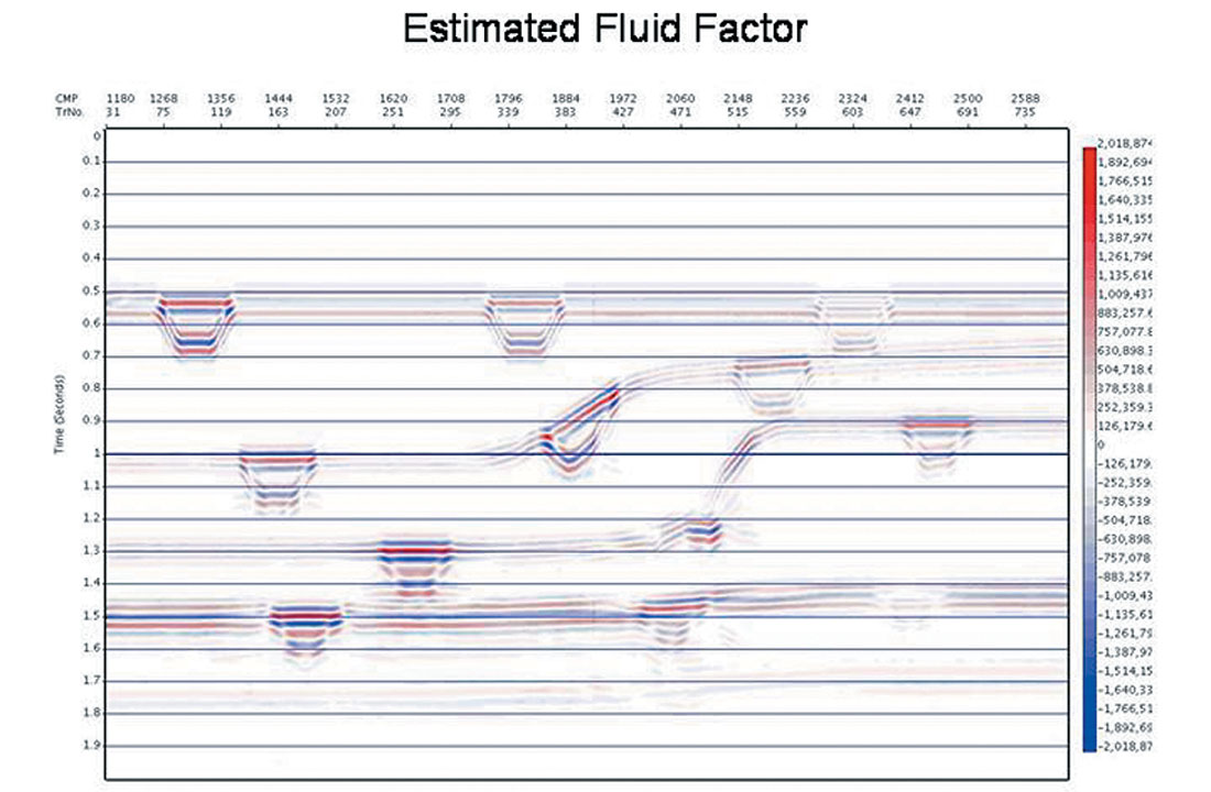
A synthetic example is shown below, in which we evaluate migration based geometrical spreading amplitude correction calculated using an interval velocity derived from the automatic time migration velocity field. As seen below, the overall model consists of a series of smooth structures for both the P and S velocity, with velocity anomalies added to the S velocity field alone (Figures 9a and b, respectively). The density is derived from the P velocity using Gardner’s rule. The example proceeds through the automatic time migration velocity and image calculation using data from finite difference elastic modeling, as shown in Figure 9c. This is followed by Dix inversion to get the interval velocity model, and a subsequent time migration produces image gathers which have been corrected for geometrical spreading. Finally, the amplitude corrected image gathers are inverted for the P and S “ zero offset” reflectivities (see Figures 9d and 9e, respectively), as per the weighted stack approach of Smith and Gidlow (Smith and Gidlow, 1987). It is noted that there should be no anomalies present in the P reflectivity section if our amplitudes and moveouts are accurate. We see only slight leakage. As in the original model, the anomalies appear in the S reflectivity section. Finally, we calculate the Fluid Factor attribute as per Smith and Gidlow, to detect all deviations of the P and S amplitudes from the Mud Rock line (see Figure 9f). This is a further demand on the accuracy of the amplitudes after time migration, and we note that the Fluid Factor amplitudes of the anomalies and smooth reflectors agree with the model.
Soft Depth: Curved and Turning Ray Migration
A diffractor travel time surface is calculated using the double square root equation with an rms velocity designated for each (time,cmp) location:

| Where: | y = | cmp location | |
| t0= | travel time to nearest surface point | ||
| x1= | horizontal distance between diffractor location and the source location | ||
| x2= | horizontal distance between diffractor location and the receiver location | ||
| Vrms(y,t0) = | rms velocity for imaging at (y, t0) |
To effect migration, integration over the entire diffractor surface on the input data is done at each (y,t0) (Schneider,1978).
In the above, the use of a single rms velocity to determine the travel time invokes the presumption of straight paths between the source and receiver and the diffractor location respectively.
However, for depth dependent interval velocity (v(z)), it is straightforward to calculate the travel time as a function of off s e t for bending or curved rays (Aki and Richards, 1980), so as to improve the definition of the diffractor response (Levin, 2003; Fowler et al., 2004). The improvement will be most noticeable for steep events, which will be improved in position and focus. In fact, the diffractor response can also be calculated to image turning rays using time migration (Fowler et al., 2004).
To illustrate curved and turning ray time migration using the interval velocity model calculated from the automatic time migration velocity, we show a synthetic and a real data example. For the synthetic data, we use a velocity model that does not vary laterally, and is increasing linearly with depth. The density model incorporates a series of layers with different densities (to give us flat reflector responses) and a salt-like body of differing density (see Figure 10a). On the top left of the model we see a snapshot of the source wavefront as it propagates into the earth. By snapshot shown in Figure 10b, we see the direction of the wavefront has changed as per Snell’s law for an increasing velocity gradient, until portions of the wavefront are propagating upward back toward the surface. We see the reflection from the salt body, with some reflection coming from the underside of the salt. The two types of reflection ray paths (curved and turning) are depicted, and for each of these types we calculate (using the Weichert-Herglotz equations (Aki and Richards, 1980) and an interval velocity model) the corresponding diffractor responses.
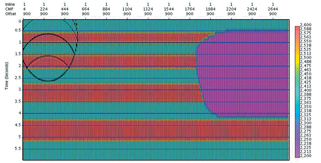
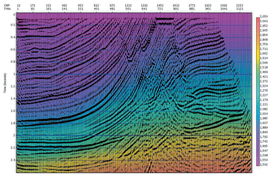
We start with Automatic Imaging using the calculated model data to determine the straight ray prestack time migration image and dense migration velocities (see Figure 11a). As straight ray migration does not correctly describe the diffractor curve for steep events in this velocity gradient model, and has no place at all in its theory for turning rays, the events near the vertical are not as well imaged and are mispositioned, and those beyond the vertical are not imaged at all.

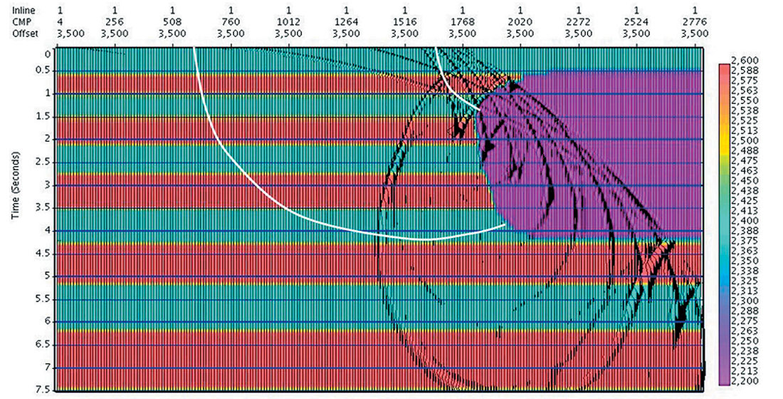
Dix inversion is then used to construct an interval velocity model from the migration velocities, and both the “curved” ray diffractor response and the “turning ray” diffractor response are calculated using this. Prestack migration is re- run to determine the curved and turning ray prestack time migration image (see Figure 11b, with interval velocity overlain in colour). Note that the imaging and positioning of the steep flank of the salt is improved, and that part of the underside of the salt has been imaged. To image more of the bottom of the salt with turning rays required longer recording times than we had actually modeled.
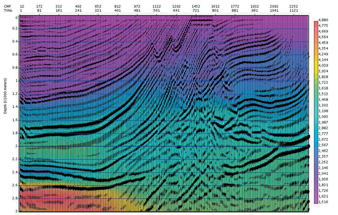
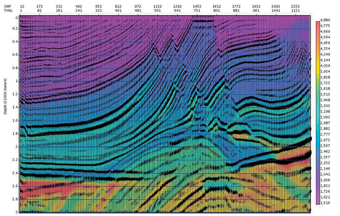
Soft Depth: Curved Ray Prestack Time Migration – Real Data Example
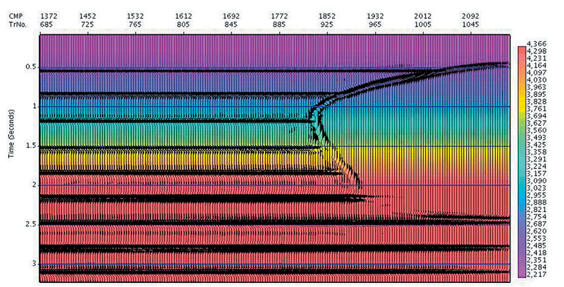
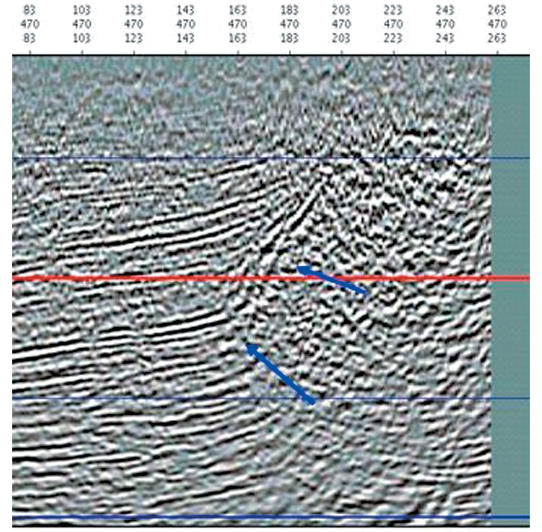
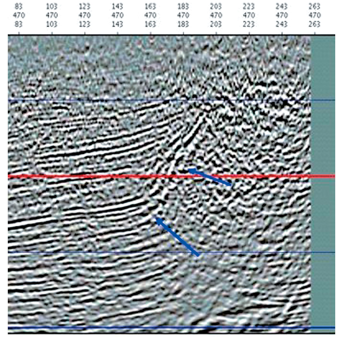
Automatic Imaging was used to produce the time migrated image cube (see a sample cross line from the cube in Figure 12a), and the time migration velocities. The velocities were inverted to produce an interval velocity cube, and the data was migrated again using travel times honouring the curved ray paths calculated from the local interval velocity (see Figure 12b). The steep flanks of the salt in the curved ray image were somewhat better focused, and also better positioned, as indicated by the improved termination of the flatter sediments against the flanks (see arrows).
Depth Migration: Marmousi
In many data sets the initial interval velocity calculated from the automatic time migration velocity will be a very good starting point for tomographic updating for continuing depth velocity refinement. For geologic regimes with slowly varying velocities (such as that of the Marmousi data set), this is expected to be the case. Shown in Figure 13a is the Automatic Image and migration velocities determined for the Marmousi data. We calculate the initial interval velocity model from the image and the RMS velocities, using the horizon constrained Dix inversion. Subsequent depth migration produced the depth image of Figure 13b (with the interval velocity overlain in colour). For purposes of comparison, the depth migration using the exact velocity model is shown in Figure 13c, with the exact interval velocities overlain.
Note that other than horizon picking on Figure 13a, the depth image and velocity model of Figure 13b has been obtained automatically. Using this model as an initial guess will likely improve the results of a subsequent tomographic search.
Conclusions
The Automatic Imaging methodology (Stinson et al, 2004) has been reviewed, with an emphasis on the optimization of quantifiable measures of image quality. Empirical testing is used to demonstrate convergence and repeatability, and real and synthetic data sets establish the benefit in velocity and imaging fidelity of this automatic, data-driven approach.
It is expected that the improved image quality as well as the fidelity and density of the time migration velocities will in turn allow for improvement in the construction of an initial interval velocity model. This is shown using “Soft Depth” applications, in which the initial interval velocity in depth is used to improve time processing applications such as True Relative Amplitude time migration and curved and turning ray time migration. The veracity of the interval velocity model is also tested for depth migration, using the Marmousi data set.
Our experience to date shows that we can routinely obtain high quality images automatically, and at a small fraction of the turn around time that is currently required to manually perform the same task.


Join the Conversation
Interested in starting, or contributing to a conversation about an article or issue of the RECORDER? Join our CSEG LinkedIn Group.
Share This Article