Past, Present, and Future applications of Geophysics in Oil Sands – Part 1

This paper is dedicated to Dr. Larry Lines (1949-2019), who was involved with seismic imaging and inversion, reservoir characterization, conventional oil and gas exploration, geophysical studies of heavy oil, oil sands, and monitoring effectiveness of steam assisted gravity drainage (SAGD), and who mentored us all. We also acknowledge the graduate students who worked on theses over the years with the University of Calgary Consortium for Research in Elastic Wave Exploration Seismology (CREWES) and Consortium for Heavy Oil Research by University Scientists (CHORUS), both groups researched the application of geophysics in heavy oil.

This paper will be published in two parts; the second part will be published in March 2022.

Introduction

In honour of the Canadian Heavy Oil Association 35th anniversary, we have authored this article on the past, present, and future applications of geophysics in the oil sands. It celebrates the early use of reflective seismic (2D, 3D, and 4D), inversion, 3C-4D seismic to identify liquid bitumen outside the steam chambers, high density seismic, and Distributed Acoustic Sensing.

Seismic data has been used extensively in the development of SAGD plays to determine the extent of wormholes in CHOPS (Cold Heavy Oil Production with Sand) (Embleton et al, 2008), and it will be a key tool for identification of where the CO₂ resides in the subsurface in CCS (Carbon Capture and Sequestration).

Oil sands can be divided into three different types:

1. Surface mining which accounts for about 20% of Canada’s oil sands deposits and are within 70 m of the surface;
2. SAGD (Figure 1), which is greater than 70 m but less than 400 m and uses well pairs with one being the injection well and the second being the production well. SAGD wells are referred to as “in situ,” and they create much less surface land disturbance.
3. CHOPS is done at a depth greater than 400 m, and the thickness of the reservoir is low.

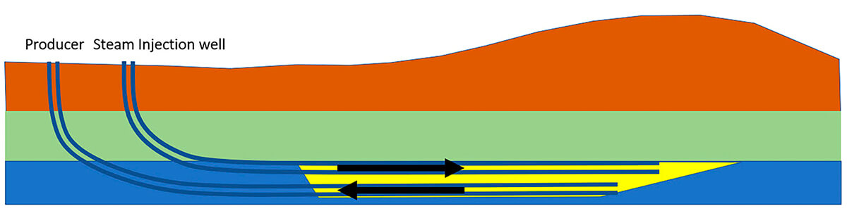
The oil sands were pioneers in using 4D because produced oil sands tend to be a Class 3 (bright spot) or Class 4 AVO, which are sensitive to fluids, especially gas – in this case, steam. The 4D seismic was used to understand the fluid flow, especially with SAGD wells, since the steam injection creates a heat front, reducing the oil viscosity and allowing it to flow. Because the viscosity is dramatically reduced, oil can flow under the force of gravity into the production well.

Historically, for oil sands, viscosity reduction has been made with steam generated using natural gas. This has resulted in large CO₂ emissions. Therefore, they have been a significant source accounting for 25% of Alberta’s GHG emissions and have become an international symbol for GHG. Recognizing this, some Canadian oil sands companies announced the Oil Sands Pathways to Net Zero Initiative to reach net-zero emissions by 2050. CCS is a practical solution that deals with GHGs emissions and has the potential to reduce opposition to oil and gas development. There is even the possibility of oil companies becoming carbon negative, e.g. https://www.cbc.ca/news/business/bakx-ccs-enhance-whitecap-david-keith-1.5884107.

This two-part article will discuss how geophysics deals with these various issues. Quite a number of advancements in geophysics have and are being made in geophysics to address these areas.

History of 2D, 3D and 4D Seismic Applications in the Oil Sands

Canada’s oil sands and heavy oil deposits are large accumulations of bitumen covering extensive areas in Alberta and Saskatchewan (Figure 2). The reservoirs are high porosity sandstones of the McMurray Formation (Athabasca Oil Sands), Clearwater Formation (Cold Lake Oil Sands), Wabiskaw Formation (Wabasca Oil Sands), Bluesky-Gething Formation (Peace River Oil Sands), and several formations like Grand Rapids, Sparky, Cummings, etc. in the Heavy Oil Belt. In Alberta, heavy oil deposits also exist in fractured limestones and dolomites of the Carbonate Triangle (Dusseault, 2002).

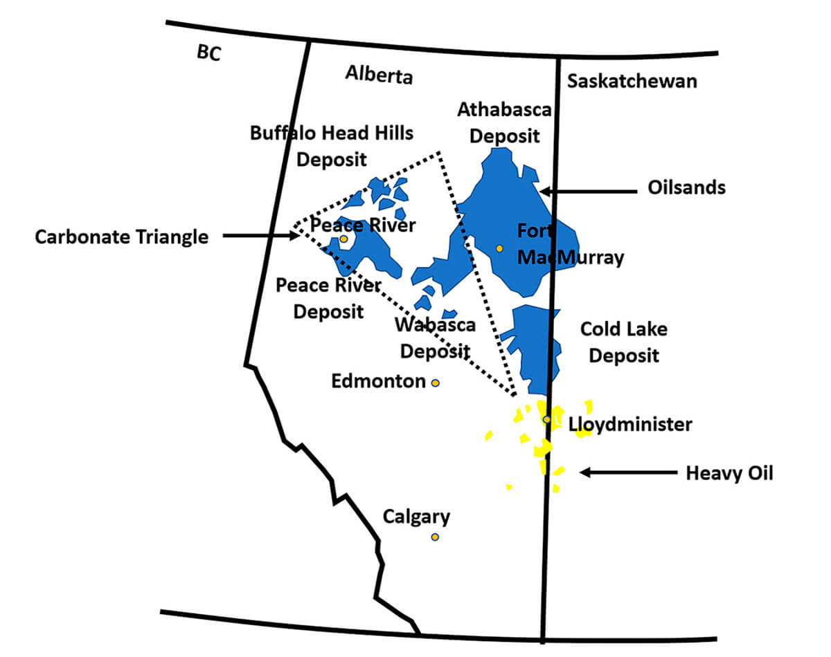
The Carbonate Triangle refers to a region delimited by the current trend of the three carbonate-hosted bitumen deposits beneath the region’s surface, forming a triangle and it is the third-largest crude reserve in the world according to the ERCB (Alberta Energy Resources Conservation Board) (Seeking Alpha, 2013a).

In Alberta, most of the bitumen deposits are contained in the unconsolidated sands of the McMurray Formation, which were deposited in a dynamic fluvial and shallow marine environment during the Lower Cretaceous. A combination of intricate channel systems, alternations of cross-bedded sands, inclined heterolithic strata (interbeds of sand and mud), massive sand sequences, and occasional concretions (calcite cemented sands) means constant changes in all reservoir properties – porosity, permeability, mineralogy, and fluid type, chemistry, and saturation (Fustic et al., 2006).

“Detailed characterization […] is required to better understand the interrelationship of components within the reservoir and the overall reservoir behaviour and reactivity at production conditions, for optimization of exploitation methods and the development of new technologies.“

In this highly complex play, understanding the reservoir with enough accuracy and detail – rocks, fluids, and their interactions and spatial variability – is essential for the optimum reservoir development planning and, consequently, to improve recovery and profitability. Integrated quantitative interpretation studies have a significant role in this planning, as they:

1. provide a more accurate, detailed, and complete model of the reservoir properties;
2. help to map the 3D distribution of lithology and bitumen;
3. define the reservoir’s small-scale architecture;
4. resolve facies and fluid ambiguities;
5. identify small-scale heterogeneities that are critical in the predictions and simulations of fluid flow;
6. use all available well, seismic data and geological information; and
7. can be updated during the life of the reservoir when time-lapse data become available.

Routine processes in these studies are techniques based on the amplitude variation with offset (AVO) or, more precisely, incidence angle (AVA). The basis of these methodologies is that the observed variation of reflectivity with angle is due to the sensitivity of seismic velocities to the rock properties such as porosity, lithology, density, fluid type and saturation, pore pressure, and textural characteristics.

AVO Analysis

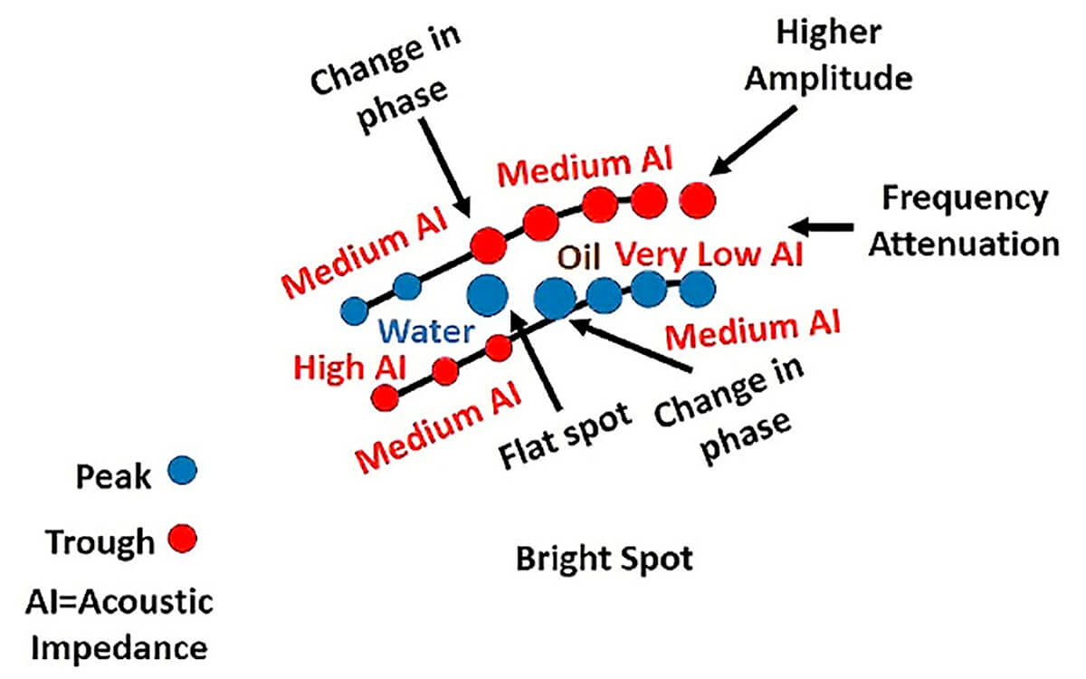
The high porosity and permeability of the oil sands can cause low impedance intervals on the well logs. These low impedance intervals correlate to bright amplitudes on processed seismic data composed of a strong trough from the top of the sand and a strong peak from the base of the sand. They are clearly visible in the full offset stacks (Figure 3).

Initially, bright spots were observed across the Pliocene/Miocene trend in the shallow waters of the Louisiana shelf in the late 1960’s and were used by Shell to de-risk plays. They were seen on 2D lines on the stacked data (Forrest, 2002). Bright spots became the basis for Amplitude versus Offset which led Ostrander (1982) to write his paper which described how the P-wave reflection coefficient at an interface separating two media is known to vary with angle of incidence, and the way it varies is strongly affected by the relative values of Poisson’s ratio of the two media (Ostrander, 1982; Castagna and Backus, 1993).

When working with bright spots, it was recognized that there were certain features in the seismic data that were related to bright spots, such as a change in phase, drop in frequency and increase in amplitude across the reservoir zone (Figure 4). This led to the development of seismic attributes to find changes in lithology, porosity, and fluid content.

2D data is used as reconnaissance, while 3D is used where we know hydrocarbons exist and is used to achieve greater resolution and imaging. One of the first 3D surveys acquired in Alberta was the Erskine 3D survey in 1978, acquired near Calgary (Galbraith, 2001).

4D seismic monitors seismic over time over a known reservoir to map changes in production and fluid flow. When acquiring a 4D survey, we begin with a base survey, and then each subsequent survey that is repeated is known as a monitor survey.

One of the first 3D 4D seismic surveys was acquired in April 1985 at the Athabasca Tar Sands Thermal Pilot. It was determined that a high-resolution 3D seismic survey was required as a base survey to locate and monitor the progress of in-situ heat fronts in a 50 m thick section of McMurray oil sands, resting on a Devonian unconformity surface, 240 m deep (Matthew et al., 1987; Zhang and Lines, 2004).

The survey area was 168 m by 196 m with 4 m by 4 m CMP bins. The seismic acquisition utilized buried seismometers at a depth of 13 m cemented in place and very light charges buried at 18 m depth. Both depths were beneath the muskeg. The seismic acquisition resulted in a minimum of 12-fold coverage except near the perimeter of the pilot area with a recording offset of 50 – 150 m (Zhang and Lines, 2004).

“3-D seismic then became used to accurately image the Devonian unconformity surface, which is a contrast from the soft sandstones of the McMurray formation to the hard carbonate-dominated geology of the Devonian, defining the distribution of this sand.”

A monitor survey was acquired in January 1987 after a four-week steam and soak period at the three production wells. Another monitor survey was acquired in April 1987 after the central injection well underwent a brief period of hot water injection before being converted to steam. A third monitor survey was recorded in November 1987 after another period of continuous steam injection in the central well (Zhang and Lines, 2004). When the first injector well was drilled, it encountered a 4 m sand aquifer directly above the erosional surface. It was assumed that this basal wet zone would influence the performance of the steam-based recovery process. Later, when drilling another well in the area, the aquifer was absent (Matthew et al., 1987). This indicated a potential problem with the proposed heating method, and the 3-D seismic then became used to accurately image the Devonian unconformity surface, which is a contrast from the soft sandstones of the McMurray formation to the hard carbonate-dominated geology of the Devonian, defining the distribution of this sand (Matthew et al., 1987).

Early interpretation of the 4D seismic utilized three seismic attributes (Eastwood, 1996; Sun, 2001; Zhang and Lines, 2004):

1. Delay time (sag) is generated by mapping the relative time difference of reflections from horizons above and below the reservoir between repeated (time-lapse) surveys.
2. Amplitudes of horizons above, below and within the reservoir between repeated (time-lapse) surveys were also used for the monitoring.
3. Frequency attenuation within the reservoir.

It was also discovered that the acoustic velocities (VP) were most affected by changes in fluid properties due to temperature. The temperature increase due to steam lowers the seismic velocity near injector wells, so the seismic velocity model can be used to delineate the effects of steam injection (Zhang and Lines, 2004).

“The temperature increase due to steam lowers the seismic velocity near injector wells, so the seismic velocity model can be used to delineate the effects of steam injection.”

Heating decreases velocities which cause horizons below the reservoir to be delayed, and with the change in velocity, we also have a change in the seismic amplitude.

CHOPS

The high porosity and permeability of the oil sands can cause low impedance intervals on the well logs. These low impedance intervals correlate to bright amplitudes on processed seismic data composed of a strong trough from the top of the sand and a strong peak from the base of the sand. They are clearly visible in the full offset stacks (Figure 3).

There are also limitations to injecting steam into the heavy oil reservoirs, especially when the reservoir is located at a depth greater than 400 m and the thickness of the reservoir is low.

In these cases, CHOPS can be used. CHOPS will fail under certain reservoir conditions, causing the loss of the well (Daniels and Schulte, 2015):

1. Wormholes that plug, collapse, or stop growing;
2. Water out;
3. Gas breakthrough; and
4. Permeability reduction from fines, formation debris, wax precipitation, and wasted solution gas.

We can utilize seismic to predict the gas breakthrough and avoid it by placing the CHOPS well at least 200 m (the theoretical maximum wormhole length) from the gas cap. The oil-gas contact is located and observed in a small number of the available wells. Using high-resolution 3D seismic data with a sample rate of 1 ms, the extent of the gas pool was defined (Daniels and Schulte, 2015).

“We can utilize seismic to predict the gas breakthrough and avoid it by placing the CHOPS well at least 200 m from the gas cap.”

The structure was defined by a depth conversion of the seismic time structure, cross-validated with the wells. The gas cap was mapped seismically and avoided through AVO analysis (Daniels and Schulte, 2015).

Seismic Inversion

With the improvement in seismic data quality from the continuous development of acquisition and processing technologies, seismic inversion has become a routine process in extracting additional information from seismic data to characterize oil sands reservoirs.

Inversion replaces an interface property, the reflectivity data, which is the contrast between the properties at the interface, into a quantitative internal rock property, such as density or elastic impedance.

“Inversion replaces an interface property, the reflectivity data, which is the contrast between the properties at the interface, into a quantitative internal rock property, such as density or elastic impedance.”

The transformation of reflectivity into rock properties is possible as the amplitude variation with offset (or angle) is a function of the Vp/Vs (monotonically equivalent to Poisson’s ratio) and P-wave, S-wave, and density contrast across the interface. These elastic properties are broadband and usually higher resolution than the conventional seismic data. They can be used to obtain:

• other elastic properties such as LambdaRho, MuRho, Lambda/Mu, density, Young’s modulus, bulk modulus, compressibility, and Poisson’s Ratio;
• estimates of petrophysical properties such as porosity, clay content, fluid saturation and lithology (e.g., Pendrel, 2001); and
• pore pressure and magnitude of principal stresses.

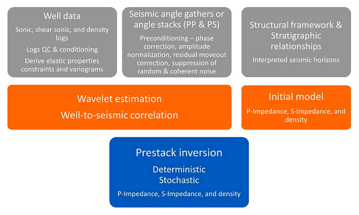
The inversion methods can be post- or prestack and either deterministic or stochastic. Poststack inversion has simpler assumptions and uses the amplitude of seismic stacked data to estimate the acoustic impedance. The prestack form uses the analysis of AVO effects on angle gathers or range limited angle stacks (PP and sometimes converted PS, in the case of joint inversion) to invert for P-impedance, S-impedance and density simultaneously. It is also the most common form of inversion currently used, as gathers contain additional information about the rock properties. The main steps in a prestack inversion workflow are:

1. Quality control/editing of well data and pre-conditioning of input seismic data;
2. Wavelet extraction and well-to-seismic correlation;
3. Initial earth model building (P- and S-wave velocities and densities), using wells and seismic mapped horizons; and
4. Prestack inversion to generate the elastic impedances and density attributes (Figure 5).

In practice, density prediction is challenging in the oil sands because of the shallowness of the data, which causes:

1. Velocity sensitivity due to a significant unconformity that exists at the base of many oil sands reservoirs in the Athabasca region (Gray et al., 2012).
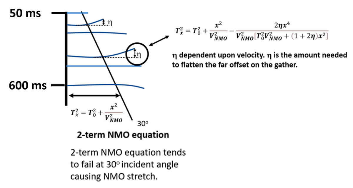
2. Vertical Transverse Isotropy (VTI), which appears as an event (peak or trough) turning upwards in the far-offsets of a gather (hockey sticking), as shown in Figure 6.
3. Horizontal Transverse Isotropy (HTI) appears as an azimuthal wobble (Gray et al., 2012; Schulte and Manthei, 2014).

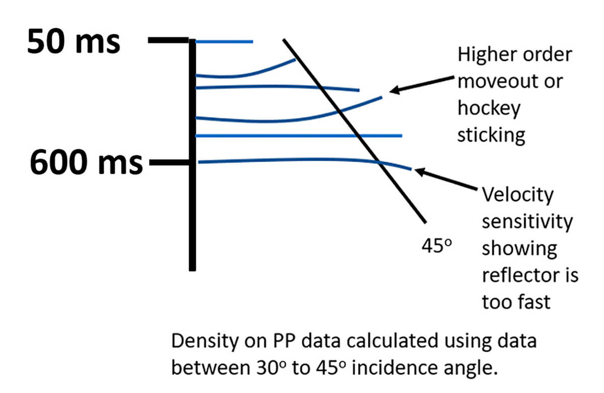
To deal with VTI, we can use a Curved Ray Prestack Time Migration or Prestack Depth Migration and higher-order moveout (Figure 7), which will use the anisotropic parameter η to flatten the hockey stick effect in far-offsets (Schulte and Manthei, 2014).

HTI or azimuthal wobble can be corrected using azimuthal moveout to flatten the wobble, which will calculate a Vslow, which is perpendicular to open fractures or the maximum horizontal stress field and a VFast that is parallel to them.

Another way to deal with these problems is to use a joint PP-PS deterministic inversion. With PS data, the density is calculated using the mid offsets where there is less noise, no hockey sticking or azimuthal wobble.

Using PP and PP-PS Data

When a conventional seismic pressure (P) wave encounters an interface, some of that energy is reflected. If it encounters the interface at an angle, some of that seismic wave induces shear on that interface, and therefore some of that energy reflects as a shear (S) wave). We call these conversions from P-to-S or PS reflections. Using converted PS seismic data, density and shear-wave impedance can be better predicted as they affect amplitudes at even small incidence angles (Zhang et al., 2018).

“Analysis of these reflection amplitudes helps us understand their sensitivity to changes in the rocks'’ physical properties and how well we can discriminate these properties from PP and PS data in the prestack domain.”

Figure 8 compares the relative contributions of P-, S-, and density reflectivity to the angle-dependent PP and PS reflection amplitudes modelled based on Fatti’s 3-term equation (Fatti et al., 1994). The two models involve a single boundary separating sand and shaly materials with their physical properties listed in the figure. These reflectivity components are fractional changes in density, and P- and S-impedance across the interface, divided by the average values of the two layers. Note that no shear or density response is induced until the seismic wave hits the interface at an angle.

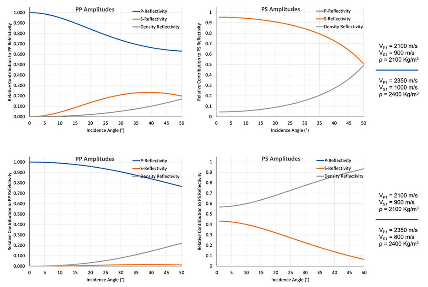
The upper layer in both cases has the same P-wave velocities and densities, but the lower layer in the second model has a lower S-wave velocity. Analysis of these reflection amplitudes helps us understand their sensitivity to changes in the rocks’ physical properties and how well we can discriminate these properties from PP and PS data in the prestack domain. For example:

• in both models, the density and S-impedance contribute more to the PS amplitudes than for the PP amplitudes;
• the density contribution is several times higher for PS, even at small incidence angles, and it can even be dominant as in the second model; and
• in some cases, the density contrast could be more important in the PS AVO signature, as shown in model two.

Interestingly, the PP amplitudes can be insensitive to changes in S-impedance across an interface, as shown by the second model, suggesting that the shear impedance could be challenging to resolve unless converted PS data are used.

The main advantages of using prestack inversion are:

1. increased resolution (better separation of interfering reflections through the removal of wavelet; reduced tuning due to the attenuation of the wavelet sidelobes (Pendrel, 2001));
2. constraints from starting low-frequency models improve the bandwidth and signal-to-noise ratio; using these a priori information from well data and seismic interpretation also involves integration with geology as a separate source;
3. improved interpretation when using elastic properties, compared to conventional seismic interpretation of seismic reflections;
4. substantially better quantitative predictions and separation of reservoir properties; and
5. possibility to quantify uncertainties.

The deterministic pre-stack inversion uses the perturbation of an initial model with P- and S-impedance and density components to compute a synthetic trace using the extracted seismic wavelet. This method iteratively evaluates the error between the input seismic trace and the computed synthetic trace until the error meets a threshold. The solution represents the model generating a minimal difference between the calculated synthetic and real seismic trace (Veeken and Da Silva, 2004). The initial model is built by interpolating well data and has a structural frame given by the shape of the mapped time horizons and known stratigraphic relationships. The role of the model is to provide the low-frequency depth trends which are below the seismic bandwidth.

The P-waves are affected by the rock matrix and the fluid filling the pore space, emphasizing fluid content, while the S-waves interact with the rock frame, emphasizing lithology. (Unless the fluid is bitumen, which has been described as a “quasi-solid” (Han and Batzle, 2008), because it has some rigidity, like Jello. The joint inversion of PP and converted PS data is more robust and stable, and it is often used because of its improved ability to characterize the lithology and fluid distribution within the reservoir. With the improved estimation of the S-impedance and density, we can have a better delineation of the hydrocarbon distribution.

“With the improved estimation of the S-impedance and density from pre-stack or joint inversion, we can have a better delineation of the hydrocarbon distribution.”

Both simultaneous and joint inversion include some form of coupling between variables, representing the regional background trends, such as relationships between logarithms of P and S impedances and between logarithms of density and P impedance (Russell and Hampson, 2006).

The band-limited nature of seismic data means that the inversion produces a non-unique solution. The inversion resolution is highly dependable on the seismic bandwidth, which in general lacks low and high frequencies. The inversion results and their derivatives are often used as external attributes in multi-attribute regression and neural network predictions to improve the resolution.

“The inversion results and their derivatives are often used as external attributes in neural network predictions to improve the resolution.”

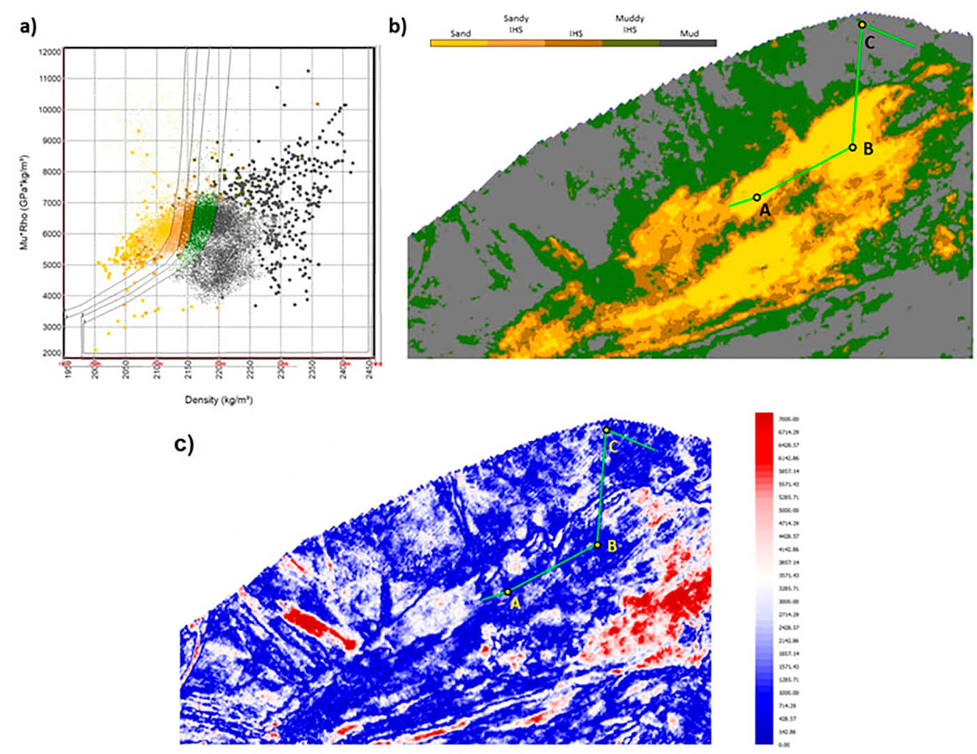
Among others, Reine (2020) showed how the inversion of PP prestack data could assist with the interpretation of a single reflection event, which can be produced by different geological elements, as for example, a sand channel, or point bar, or mud plug. He showed that the resulting density obtained from the simultaneous inversion was consistent with the well data and noted that a significant density difference between two wells B and C could produce similar amplitudes of stack data at the two locations (Figure 9).

For the oil sands reservoirs, density is critical to discriminate between facies types with varying amounts of clay content because higher clay content corresponds to higher density. For the case shown in Error! Reference source not found., using a crossplot of MuRho -Vs²*ρ vs density allowed the interpretation of well facies on the equivalent seismic properties obtained from simultaneous inversion (Figure 10). Interesting to note is that the facies interpretation from well and seismic data produces a clearer geologic picture than the amplitudes.

The spatial heterogeneity of the heavy oil deposits and the thin, intra-formational shale layers can be challenging as their thickness is finer than the deterministic inversion’s vertical resolution. An alternative approach is a stochastic or geostatistical inversion, which removes some of these limitations by simulating multiple scenarios (realizations) having the same result at the wells but with vertical and lateral variability beyond seismic resolution. The vertical and horizontal variability is constrained by mathematical functions called variograms, which are spatially varying statistics obtained from well data, and in the case of these inversions, the seismic data too.

An alternative approach is a geostatistical inversion, which removes some of these limitations by simulating multiple scenarios (realizations) having the same result at the wells but with vertical and lateral variability beyond seismic resolution.

The geostatistical method reduces the non-uniqueness of the inversion process because all realizations satisfy the observed seismic data and therefore are equally possible. The process only constrains the high frequencies. Averaging all realizations will result in a similar result as that of the more commonly used deterministic inversion (Delbecq and Moyen, 2010). The number of high-frequency realizations is determined by the variograms and the number of layers in the initial model (the stratigraphic grid). The stochastic realizations can be combined, based on various statistical geometric criteria such as sand or shale thickness or lateral extent, to estimate probability cubes, which can be selected to interpret different scenarios.

Figure 11 shows a schematic representation of the frequency spectra of the deterministic and stochastic results:

• in deterministic inversion, the frequency spectrum includes a low-frequency component obtained from the well’s depth trends. A seismic bandwidth component shows layering patterns close to the upper frequency limit of the seismic data; and
• in stochastic inversion, the statistical well information generates a higher frequency component beyond the upper seismic frequency, but constrained by variograms determined from seismic and wells, in the form of micro-layering at a sub-seismic scale.

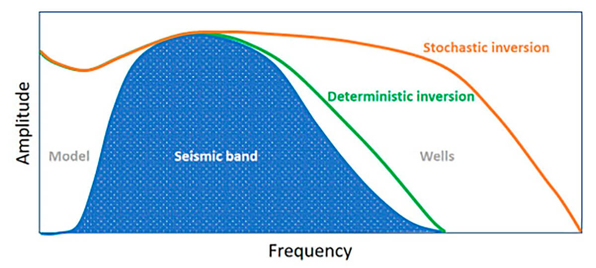
Each inversion scheme has its advantages and limitations, with deterministic inversions being robust even in the presence of poor data, and stochastic inversion having increased resolution and quantified uncertainties. The increased vertical resolution of the stochastic inversion could provide a more accurate distribution of the reservoir elastic properties. In turn, it will produce a more detailed facies distribution and better estimation of reservoir connectivity. Detection of small-scale elements such as thin shale layers within the inclined heterolithic strata (IHS) is critical. They can constitute barriers in reservoir development and are more challenging to resolve. The seismic bandwidth and their thickness and seismic velocity control their detectability (Zhang et al., 2012).

Usually, the inversion is performed in conjunction with the quantitative interpretation of reservoir properties and lithology classification. This step connects the inverted elastic properties to more understandable reservoir properties such as porosity, saturation, clay content, and lithology.

“Usually, the inversion is performed in conjunction with the quantitative interpretation of reservoir properties and lithology classification. This step connects the inverted elastic properties to more understandable reservoir properties such as porosity, saturation, clay content, and lithology.”

However, one of the challenges of extracting the reservoir properties from the AVO signatures is that the relationship between the reservoir physical properties and elastic properties obtained from inversion is non-unique. Ambiguity can occur between various lithologies, porosity, and fluids. For example, shales could mimic the seismic signatures of uncemented sands, or heavy oil with dissolved gas could have similar properties as freshwater sands (Reine, 2017). In contrast, clean and slightly cemented sands can have a distinct seismic response different than clean oil-saturated uncemented sands, even when they have comparable porosities and composition (Avseth et al., 2013). One option to resolve these types of sedimentological variations is to combine inversion with rock physics modelling. The rock physics model of the reservoir will add constraints from the known petrophysical properties and their local expected change.

Conclusions for Part 1

AVO techniques have a tremendous utility in the characterization of the oil sands reservoirs, despite the myriad complications affecting the seismic amplitudes (some of them discussed here). Experience has shown that one of the most robust strategies is integrating the seismic reflection data with AVO inversion and rock physics modelling. The key properties in the facies analysis are the density and Vp/Vs. They are lithology-dependent, with bitumen sands having higher densities and lower Vp/Vs and shales having lower densities and higher Vp/Vs. These properties, determined from seismic data, have proven to be very useful in delineating oil sands reservoirs.

This is the end of the first part, the second part will be published in March 2022.