Prestack Waveform Inversion Using a Genetic Algorithm – The Present and the Future

Abstract

Use of prestack data for quantitative analysis of hydrocarbon reservoirs has gained popularity over the past decades. Most of these quantitative studies rely on the seismic reflection amplitude variation with offset or AVO analysis. AVO makes a simple assumption that every reflection event on the prestack seismic data is a primary P-wave reflection, and there is no contamination of these amplitudes from other wave modes. Using synthetic data for a finely layered elastic model, it is demonstrated that such simple assumptions are incorrect, and there is a lot of interference of P-wave reflection amplitudes with other wave modes, especially at high offsets/angles. To properly model such interference, a full-waveform prestack inversion must be used. Such a prestack inversion has been successfully used in a continuous prestack inversion, in a hybrid inversion scheme, and in geo-hazard studies like pre-drill pore-pressure prediction and shallow water flow analysis.

Prestack inversion is computer intensive, since it must compute many forward synthetic models to obtain an estimate of the optimum earth model at a given common midpoint (CMP) location. This limits application of this inversion method to geologically simple areas with little structural complexity. As the computers are becoming faster every day, it is expected that in the near future it will be possible to efficiently compute forward prestack seismograms for complex models, and apply prestack inversion over geologically complex areas.

Prestack inversion examples presented here use P-wave seismic data only. An attempt to use converted wave data in conjunction with P-wave data in a multicomponent prestack inversion scheme demonstrates that the multicomponent inversion can obtain a more accurate model than the P-wave inversion alone. In addition, multicomponent inversion can be easily extended to incorporate anisotropic earth models. It is therefore expected that in the future, prestack inversion will be extended to multicomponent seismic data to allow extraction of anisotropic earth models.

Introduction

The use of prestack seismic data as a tool for quantitative analysis of hydrocarbon reservoirs has become very popular in the geophysical industry over the past two decades. Study of seismic reflection amplitudes as function of source-to-detector offset has emerged as a new technology, known as the amplitude-variation-with-offset (AVO). Following the pioneering works by Ostrander (1984), Shuey (1985), Smith and Gidlow (1987), Rutherford and Williams (1989) among others, AVO is now routinely used for reservoir evaluation. An excellent collection of papers on the advances of AVO technology can be found in Castagna and Backus (1993). Conventional P-wave AVO analysis has also been extended to multicomponent data to include information from converted reflections. Mallick et al. (1998) studied the P-wave AVO in different azimuthal directions to find that the P-wave AVO is sensitive to the principal anisotropy directions.

In spite of all the developments noted above, the AVO technology suffers from a fundamental drawback. AVO and related methods make a simplified assumption that every event on prestack seismic data is a primary reflection and there is no contamination of these events from mode conversions and multiple reflections. Such an assumption may be true for simple models with a few layers, separated by large intervals. In reality, such an assumption is too simplistic, and reflection events on real seismic data are in fact contaminated by wave-modes other than primary reflections. Since AVO is fundamentally an amplitude related method, contamination of primary reflections by other wave-modes can significantly affect the AVO results. This is demonstrated in Figures 1 and 2.

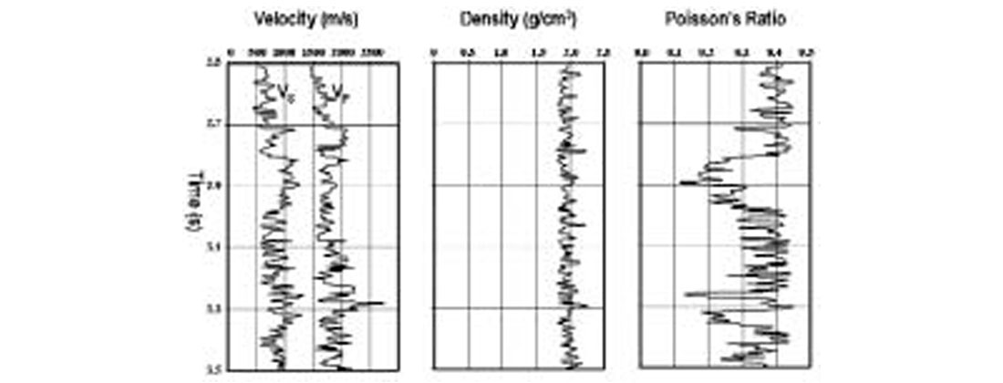
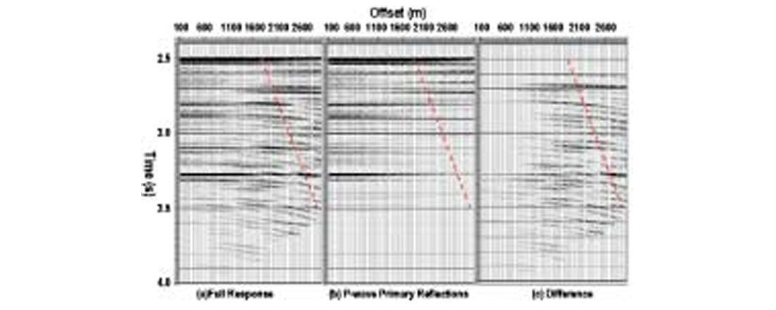
Figure 1 is an elastic earth model, and the synthetic seismograms computed using this model are shown in Figure 2. Figure 2a shows the full waveform synthetics that include all wave-modes. Figure 2b on the other hand shows the synthetics computed using P-wave primary reflections only. Figure 2c is the difference of the synthetics shown in Figures 2a and b. All the synthetic traces in Figure 2 are plotted with the same normalization so that their amplitudes can be compared directly with one another. The dashed lines on Figure 2 represent the x = z lines, i.e. the lines along which the offset is equal to the target depth. Figure 2 clearly demonstrates that primary reflections can be seriously contaminated by interference from other wave-modes, especially at high offsets. Even if the use of prestack traces is limited to x = z, there could be substantial interference of primary reflections with other wave-modes. Recently, there has been a lot of interest in the AVO inversion to high angles for getting the density contrast (Kelly et al., 2001; Skidmore et al., 2001). Such an inversion requires traces beyond x = z, where primary reflection amplitudes are heavily affected by the interference from other wave-modes. AVO inversion to these offsets will give incorrect results unless the amplitudes are compensated for these interference effects. Most of these interference effects are due to converted wave reflections and interbed multiple reflections, resulting from the seismic wave propagation in finely layered media. They are real, and no seismic processing method can remove them entirely from the data. In order to properly account for the interference of primary reflections with other wave-modes it is necessary to use a methodology that can correctly account for their effects, and this can only be achieved by prestack waveform inversion.

Prestack Waveform Inversion

Although prestack seismic data can be inverted in many different ways, the method that will be discussed here is a non-linear elastic inversion methodology, based on a Genetic Algorithm (GA) optimization. An account of different geophysical inversion methods can be found in Treitel and Lines (2001), and an account of different methods for prestack seismic inversion is given in Sen and Stoffa (1991) and Mallick (1995).

GA is a Monte-Carlo type (Press, 1968) optimization procedure that uses the analogy of the biological evolution in directing its search process in the model space. The prestack GA inversion used in this paper is described in detail by Mallick (1999). In essence, this methodology takes prestack seismic data as input and uses GA search algorithms to obtain an estimate of the elastic earth model (Figure 3). Note that the input to GA inversion is prestack seismic data that is not corrected for the normal moveout (NMO). Since the NMO velocities and AVO behavior on prestack seismic data are simultaneously searched during the prestack GA inversion, the method provides both low and high frequency components of the elastic earth model. In addition, to properly account for all the interference effects, the inversion uses an accurate modeling methodology that includes primary, converted, and multiple-reflected wave-modes. Such an accurate modeling method leads to a very accurate estimation of the elastic earth model to a resolution of 1/4th to 1/6th wavelength of the dominant frequency of the seismic data (Mallick, et al., 2000).

Applications of Prestack Waveform Inversion

Prestack GA inversion has been successfully applied in continuous prestack inversion, hybrid inversion, and geo-hazard studies such as pore pressure prediction and shallow water flow (SWF) prediction.

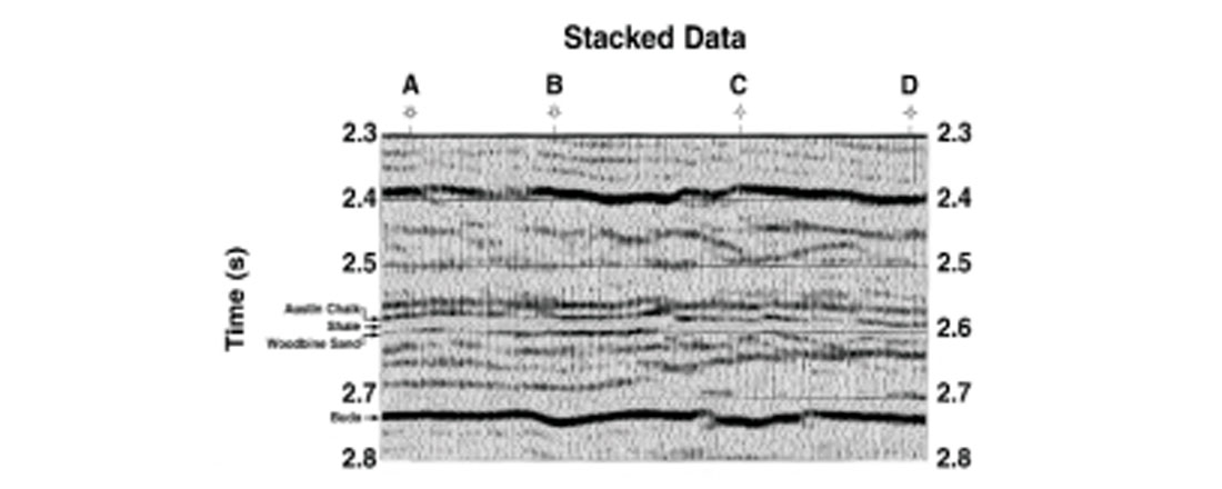
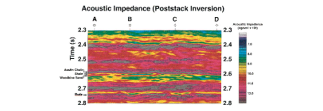
Continuous prestack inversion: In continuous prestack inversion, common midpoint (CMP) ordered prestack seismic data over a seismic line are inverted. Figure 4 shows a stacked seismic section from a Woodbine sand gas field, east Texas. The Woodbine formation consists primarily of a sand/shale package of late Cretaceous age that was deposited under a deltaic environment on top of the Buda carbonate shelf margin, and it underlies the Austin Chalk formation. Primary interest in the Woodbine package is the sand layer, known as Woodbine sand that appears as a toplap pinchout against a shale layer. This shale layer, in turn, underlies the Austin chalk formation. The Austin chalk, shale, Woodbine sand, and Buda formations are marked on Figure 4. Out of four wells, marked A, B, C, and D in Figure 4, wells A and B produce gas from the Woodbine sand whereas wells C and D were dry. At well A, the P-wave sonic and density logs were only run over the Austin chalk, shale, and Woodbine sand formations. At well D, the P-wave sonic and density logs covered a time window of 2.3s down to the base of the Woodbine. Finally, no sonic or density information were available in wells B and C. Using the well information at A and D, both poststack and prestack inversions were run on the data set. Figures 5 and 6 show the acoustic impedance obtained from these inversions. A comparison of these two figures clearly shows the superiority of prestack inversion over poststack inversion. The Woodbine sand is far clearer in Figure 6 than in Figure 5. In addition, Figure 6 also shows the presence of Woodbine sand at producing well locations A and B and its absence at dry well locations C and D much more clearly than does Figure 5. More details on the comparison between poststack and prestack inversion on the Woodbine sand data were given in Mallick (1999).

Hybrid Inversion: Although prestack inversion gives far superior results than poststack inversion, it must be noted that prestack inversion is computer intensive. In spite of its superiority, it is therefore difficult to apply prestack inversion on a routine basis on large data volumes. To handle large volumes of data, prestack inversion must be run in conjunction with poststack inversion in a hybrid inversion scheme (Mallick et al., 2000). In hybrid inversion, prestack inversion is run only at selected control point locations. From the elastic earth models, obtained from prestack inversion, P- and S-wave impedance values at those control points are calculated. Note that prestack inversion finds both low and high frequency models. Consequently, P- and S-wave impedance from prestack inversion can be used to constrain the low frequency impedance trend for poststack inversion. Therefore, in a hybrid scheme, once P- and S-wave impedance from prestack inversion are obtained, a standard AVO analysis method is applied on the prestack seismic data to compute the AVO intercept and gradient traces. Amplitudes of AVO intercept traces are proportional to the P-wave normal incidence reflectivity. Under the assumption of a background P-to-S velocity ratio (VP/VS), AVO intercept and gradient traces are then combined to obtain pseudo S-wave traces (Mallick et al., 2000). The amplitudes of such pseudo S-wave traces are proportional to the S-wave normal incidence reflectivity. Once the traces that are proportional to the normal incidence P-wave (AVO intercept) and S-wave (pseudo S-wave) reflectivity are obtained as above, two poststack inversions are run as follows:

1. AVO intercept traces are inverted using the P-wave impedance from control points as low frequency impedance trend. This gives the P-wave impedance for the entire data set.
2. Pseudo S-wave traces are inverted using the S-wave impedance from control points as low frequency impedance trend. This gives the S-wave impedance for the entire data set.

Once the P- and the S-wave impedance values are obtained, they can be combined to get other attributes such as V_P/V_S, Poisson’s ratio, Lamé attributes (λρ, μρ) etc.

Hybrid inversion provides an elegant way of using inversion as a reconnaissance exploration tool in developing new areas with sparse or no well control (Mallick et al., 2000). In a standard poststack method, inversion results are influenced by the low frequency trend from the well information. When well control is sparse, low frequency impedance trends from these sparse locations are interpolated for the entire data range as a guide to the poststack inversion. In the event of rapid changes in the low frequency trend, poststack inversion will give incorrect results. In hybrid inversion on the other hand, the user can control the required number of control points, depending upon the complexity of the geology and depositional history, leading to an accurate inversion result. In addition, the hybrid method allows estimation of both P- and S-wave impedance that is not possible in a standard poststack method unless Shear wave logs are available.

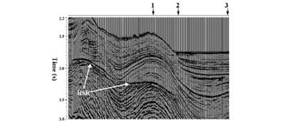
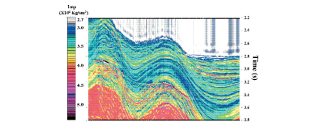
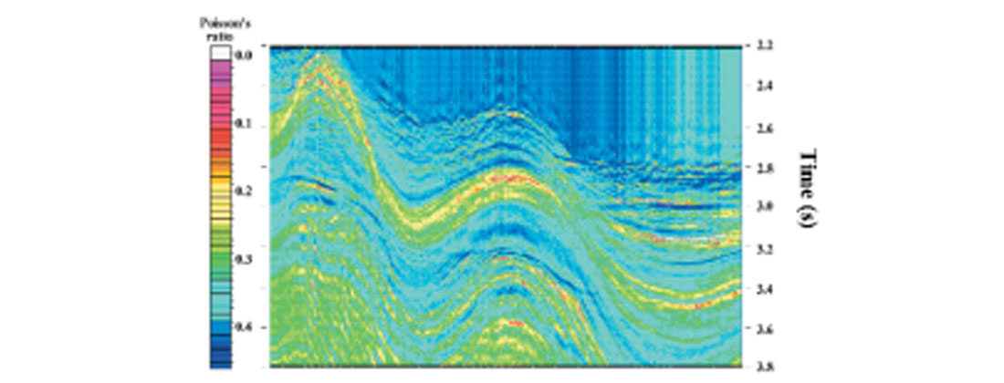
Figure 7 is a stacked seismic section from the deep-water Andaman Sea, offshore India. The zone of interest in this data set is the region below the gas hydrate layer, characterized by a bottom- simulation reflector (BSR) as marked. BSR is typically found in a deep-water environment and it is believed to be the boundary between the methane in a solid hydrate phase above and gaseous phase below. The purpose of this investigation was to find if any evidence of free gas underneath the BSR could be detected by hybrid inversion. Three control points where prestack inversion was run to constrain the low frequency impedance trends are marked with arrows in Figure 7. Figures 8 and 9 show the P- and S-wave impedance sections from the hybrid inversion. Figure 10 is the Poisson’s ratio section, computed from the impedance values of Figure 8 and 9. A close look at Figure 10 shows the evidence of free gas below the BSR where the Poisson’s ratio drops to the 0.1-0.15 range. Details on the hybrid inversion were published by Mallick et al. (2000).

Geo-Hazard Application: Elastic earth models obtained from prestack inversion have been very useful in geo-hazard studies such as pore pressure prediction and shallow water flow (SWF) analysis (Gelinsky, 2001, De Kok et al, 2001; Khan et al., 2001).

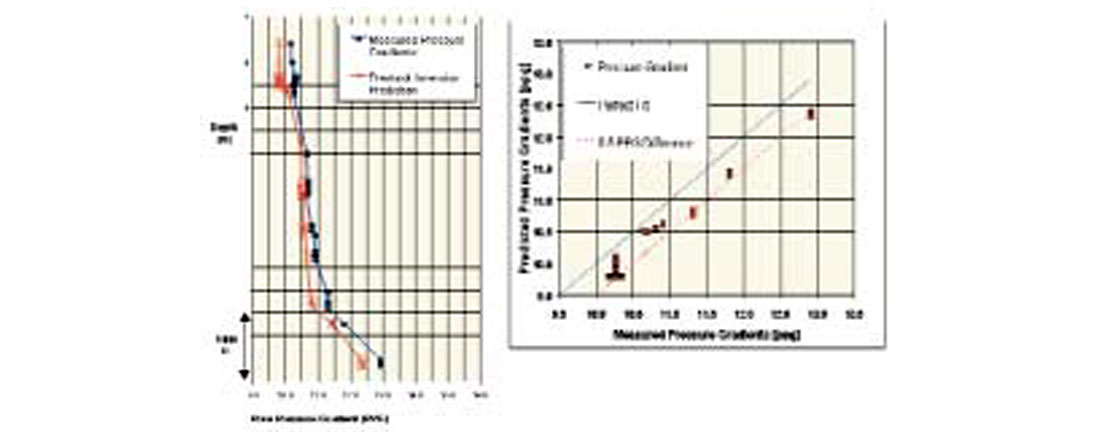
Pressure prediction prior to drilling using seismic stacking velocities has been well known for quite some time. Seismic velocities that are slower than a normal velocity trend are indicative of overpressured formations (Eaton, 1972). By the process of matching all the details in the observed data, prestack waveform inversion can obtain an elastic model that resembles closely the actual well information. P- and S-wave velocities, obtained from such prestack inversion has been successfully used in developing a rock model and predicting pore pressure (Gelinsky, 2001; Khan et al., 2001). Figure 11 is an example of such a pore pressure prediction. Notice that the pore pressure gradients, predicted from the prestack model, are within 0.5 pounds per gallon (ppg) from the actual pressure gradients measured in the wells.

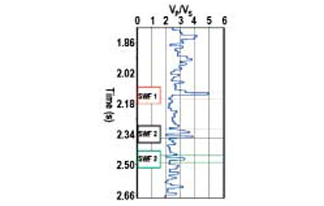
SWF occurs in a deep-water environment and is caused by highly pressurized water pockets, resulting from a rapid deposition. These SWF layers are potential drilling hazards, therefore identifying them prior to drilling is important in well planning. Since SWF layers typically have almost identical acoustic impedance as the surrounding formations, it is difficult to identify them on the stacked seismic data. However, because these SWF layers are mostly water bearing, they are characterized by a high value of VP/VS, and it is possible to identify them by prestack inversion. De Kok et al. (2001) and Khan et al. (2001) have run prestack inversion over a known SWF area in the deepwater gulf of Mexico, and could successfully identify all SWF layers from their inverted results (Figure 12).

The Way to the Future

Prestack inversion has a wide application in different aspects of reservoir characterization and pre-drill geo-hazard analysis. Considering the potential of this method, it is expected that in the future prestack inversion will be used more widely than it is used today. As noted before, prestack inversion is computer intensive, and the primary reason for this is the fact that the inversion must compute millions of prestack forward models at every CMP location (Mallick, 1999). Therefore, an efficient forward modeling algorithm plays a major role in the use of prestack inversion. In the inversion examples shown here, an efficient forward modeling algorithm for horizontally stratified media using a reflectivity method (Fuchs and Müller, 1971) has been used. The primary reason for using a reflectivity method is discussed in detail by Mallick (1999). In essence, this method computes a very accurate seismic response from a finely layered medium fairly quickly. This is not possible with other fast modeling methods such ray tracing. To accurately model the details of all stratigraphic features that are usually needed in prestack inversion, an accurate modeling of the seismic response through a finely layered medium is absolutely essential. However, notice that the reflectivity method is strictly valid for a horizontally stratified medium. In the event of dipping events, the data must be prestack time migrated prior to inversion. Such a procedure is acceptable when the geology is not too complex. However in areas of complex geology, using the reflectivity method for forward modeling may not be valid, and it may be necessary to use a modeling algorithm such as a finite difference method. Running a finite difference modeling millions of times at every CMP location as prestack inversion demands, is theoretically possible, but will take an enormous amount of time, even with the fastest present day computers. However, computers are getting faster every day, and we may not be far from running finite difference modeling to handle complex geology in prestack inversion.

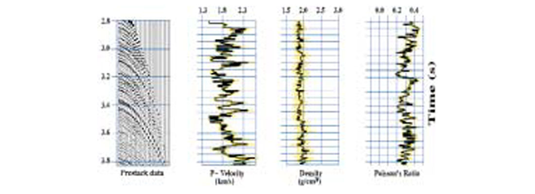
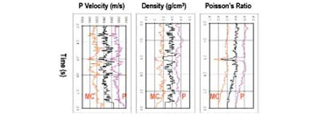
Inversion examples presented here used P-wave data only. Although P-wave velocity can be obtained quite accurately in such an inversion, it must be noted that the estimation of S-wave velocity is obtained indirectly from the variation of P-wave reflection amplitudes as functions of angle of incidence. In addition, estimation of density from P-wave inversion is not very accurate. This is evidenced by the larger errors in the estimation of density in comparison to the estimation of other parameters in Figure 3. If P-wave as well as mode converted reflections are simultaneously inverted using multicomponent data, it is expected that the elastic model extracted from such multicomponent inversion should provide a more accurate model than the P-wave inversion alone. Figure 13 is an example of multicomponent prestack inversion on synthetic data, created from a real well log. Note that the density is much better resolved in multicomponent inversion than in P-wave inversion. An accurate estimation of density in addition to P- and S-wave velocities plays a very important role in discriminating between producing and nonproducing reservoirs (Mallick, 2000; Kelly et al., 2001; Skidmore et al., 2001). Therefore, multicomponent inversion is expected to gain popularity in the future.

So far, all the inversion methods described above were for isotropic earth models only. Although the assumption of isotropy may be adequate in P-wave inversion, for the multicomponent inversion it may be essential to consider anisotropic earth models in order to explain all features in the observed seismic responses. This is primarily due to the fact that the S-waves are much more sensitive to anisotropy than the P-waves (Thomsen, 1988). In addition, both P- and S-wave reflection amplitudes are sensitive to anisotropy. Inversion for anisotropic models for transversely isotropic media with a vertical axis of symmetry (VTI medium) has been attempted with some success by Grechka et al. (2001). Multicomponent inversion can be extended to incorporate anisotropic earth models quite easily (Mallick, 2000). It is therefore expected that future developments in multicomponent inversion will allow inversion for anisotropic earth models.

Conclusion

Prestack inversion is a valuable exploration tool than can be effectively used in reservoir characterization and pre-drill geohazard studies prior to well planning. Since prestack inversion correctly handles the interference of primary reflection events with other wave-modes, it generates a very accurate model of the earth that is not achievable in a traditional AVO analysis. The potential of prestack inversion is enormous, and it is expected that this method will find wide use in future exploration of hydrocarbon reservoirs.

Acknowledgements

I thank our clients who gave permissions to use their data sets shown in this study. I also thank WesternGeco for permission to publish the paper. Finally, I thank Laurent Meister and Mark Egan for critically reviewing the manuscript and suggesting many improvements.