Propagation of borehole derived properties via a Support Vector Machine (SVM)

Introduction

Rock mechanical properties are an essential piece of information for applications like borehole instabilities analysis during drilling. It is estimated that borehole instability problems cost the oil industry worldwide about 1.0 billion dollars per year (Erling, et al., 1996).

Traditional methods of propagating mechanical properties from a given borehole to a proposed borehole are based on parameter shifting and spatial interpolation. The validity of these methods, in general, decreased when dealing with a sparse and distant collection of boreholes. The propagation of rock properties in these situations carries a significant amount of risk. Fortunately, seismic data possess high lateral resolution, and therefore, it can be used in conjunction with borehole data to propagate borehole-derived properties to an area of interest. In this paper we present an algorithm based on a Support Vector Machine (SVM) that is capable of propagating sparse measurements obtained at borehole locations to a 2-D/3-D volume where seismic data exists.

SVM has been gaining popularity in regression and classification due to its excellent performance at the time of dealing with sparse inputs (Vapnik, 1998). The idea behind SVM is quite simple. During the training (learning) phase, the SVM will develop a functional mapping between an input vector (seismic attributes) and a target output (known rock physical properties at borehole locations). The functional is later on used to predict rock physical properties at locations with unseen targets where only seismic attributes are known.

Support Vector Machine

Given a set of seismic attributes (estimated from post-stack or pre-stack volumes) { x_n , n=1,…,N } along with the corresponding rock property targets { t_n , n=1,…,N } from several boreholes. The SVM makes predictions based on a function of the form:

where {ω_n} are the model weights, and K(x,x_n) denotes the kernel function (Schölkopf et al., 1999). Table 1 provides examples of kernel functions that have been extensively tested in the machine learning literature (Vapnik, 1998). We notice that an important feature of equation (1) is that the kernel function defines one basis function per training set. This is an important difference with respect to classical regression analysis where the basis functions are independent of the training set. A simple example is fitting a straight line to a set of observations; the functional model has the following form y = ax + b regardless of the (x_n , y_n) input pairs. During the learning stage, a set of input-target pairs is used to find the model of dependency of the targets on the inputs. Please, notice that in this paper vector quantities are identified with bold fonts, for instance x_n represents a vector of attributes at time sample n, the amplitude of the seismic waveform is one possible attribute. It is clear that the learning stage involves the estimation of the appropriate weighting parameters {ω_n}.

Bayesian Estimation of {ω_n}.

We first assume that we have access to a dataset of input and target pairs {x_n , t_n ; n=1,…,N}. Furthermore, we will assume that the targets are contaminated by observational errors:

To avoid notational clutter we will re-write equation (2) in matrix form:

where Φ denotes the design matrix composed of rows that are given by ϕ(x_n)=[1,k(x₁, x_n),k(x₂, x_n),…,k(x_N , x_n)]. The vector of targets is given by t, and finally, ω indicates the vector containing the unknown weights.

We will follow Tipping (2001) and utilize a Bayesian procedure to estimate the weights. In addition, it is important to stress that the Bayesian framework can also be used to estimate the noise level in the targets and the important hyperparameters that define the tradeoff between excessive fitting and simplicity of the regressor given by equation (1). We will come back to this point when fully describing the algorithm.

In Bayesian inference we construct the a posteriori probability distribution of the unknown vector of parameters ω given the targets (data) and prior information about the unknowns (Ulrych et al., 2001). In our case the posterior is given by

where p(t|ασ) indicates the data likelihood. If we assume that the errors are normally distributed and uncorrelated:

The prior p(ω|α) is selected according to the following assumptions. First we assume that a Gaussian distribution can model the a priori distribution of each individual weight. We will also assume that the weights are uncorrelated. Furthermore, we will assume that each weight has associated to it an individual variance. If we define the variance of each weight by ω_k, then it is easy to show that the prior becomes:

The denominator in equation (4) represents a normalization constant and will not enter in the estimation of the model vector of weights. So far we have defined the a posteriori probability. This probability depends on two (unknown) hyper-parameters: α,σ². First, we will assume that the hyper-parameters are known. In this case, we can find the maximum a posteriori (MAP) solution of the problem. This is the vector ω that maximizes the a posteriori probability. It is quite simple to show that to maximize the a posteriori probability is equivalent to minimizing a quadratic cost function of the form (Ulrych et al., 2001):

The MAP solution (the minimizer of equation (7)) is given by:

Notice an important consequence that arises from our analysis. The diagonal term in equation (8) is a generalization of the well-known ridge regression term or damping term used to guarantee the stability of the inverse of Φ^ΤΦ (Lines and Treitel, 1984). In fact, if α_k=c,k=1,…,N, then equation (8) becomes:

The disadvantage of expression (9) resides in the fact that the solution vector tends to have entries that are all different from zero. It is interesting to notice that by assigning an individual variance to each element of the vector of unknowns, we are implicitly demanding a solution with a certain degree of sparseness. In other words, if not all the weights are needed or relevant in fitting the targets why should we use them?. Tipping (2001) called this particular approach to the inversion of equation (1) the Relevance Vector Machine (RVM). This name emphasizes the fact that only a few relevant basis functions are needed for the design of the SVM.

So far we have obtained the maximum a posteriori solution (8) based on two chief assumptions: the variance of the noise σ², and the vector α are known. It is clear that this is often not true. An attractive feature of the Bayesian framework is that it also provides a strategy for hyper-parameter estimation. For this purpose we use the integrated likelihood function of the data (the targets) given the hyper-parameters. Since we have adopted Gaussian distributions to describe both our data likelihood (5) and the a priori distribution of parameters (6), the integrated likelihood can be solved analytically (Mackay, 1992, Tipping, 2001):

To obtain α and σ we differentiate equation (10) with respect to the hyper-parameters and we perform an alternate maximization of equation (10). The process is continued until convergence is achieved. It is interesting to note that during the optimization process some elements of the vector α will become very large. In other words, the variance associated to one or more weights ω_k, σ_k²=1/α_k, becomes small. This implies that some elements ω_k can be pruned (set to zero). This is quite similar to the problem of designing high resolution Radon Transforms for de-multiple (Sacchi and Ulrych, 1995) and high resolution Fourier Transforms for the interpolation of irregularly acquired and gapped data (Sacchi et. al, 1998). In these particular applications, a sparse distribution of model parameters is sought as a mean of improving the resolution of linear operators such as the Radon Transform and the Fourier Transform. We must stress, however, that in the present application, a Gaussian prior with variable variances is used to achieve the same effect. The difference between using the aforementioned approach versus the sparse inversion methodology introduced in Sacchi and Ulrych (1995) is under investigation.

Example

As stated above, the incorporation of seismic information to the property propagation process confers an important advantage because it enables the incorporation of geological constraints and lateral variations to the propagating solution. However, defining empirical relations between borehole properties and seismic attributes may require a correct depth-to-time conversion, and more importantly, requires a physical bridge to connect seismic attributes and borehole properties. By using SVM one attempts to encode all the complexity of the regression process in the Kernel function by defining one basis function for each training set.

In our numerical tests we have developed a functional to map seismic amplitudes to P-wave velocities by training a SVM with the already presented Bayesian strategy. Our working scheme is summarized as follows:

1. Select a corridor of interest in the seismic section and borehole-derived properties at locations within the seismic volume.
2. Extract post-stack seismic attributes from stacked CMP gathers adjacent to the targets (In our case P-wave velocities derived from sonic logs).
3. Use the Bayesian algorithm outlined above (Mackay, 1992; Tipping, 2001) to train the SVM.
4. Use the SVM as a regressor to propagate the desire velocities to new spatial locations in the seismic volume.

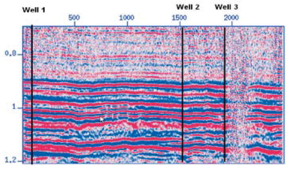
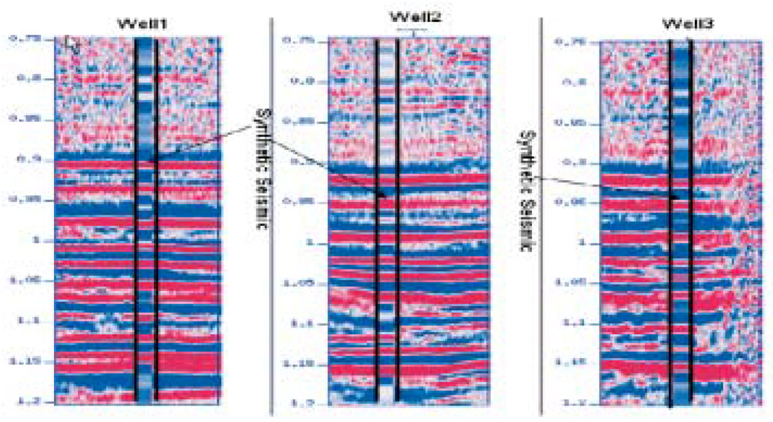
We illustrate the performance of the proposed method with a real seismic dataset. We will attempt to propagate compressional velocities but it is clear that other rock mechanical properties, such as Young’s Modulus and Lame Parameter, can be propagated using this scheme. Figure 1 portrays a seismic corridor (stacked section) and the location of three wells. The boreholes, at CDP positions 148, 1523 and 1911 were used to compute reflectivity sequences, synthetic traces, and to extract our targets (P-wave velocities versus two-way traveltime). In Figure 2 we portray the synthetic seismic traces obtained from the reflectivity sequences.

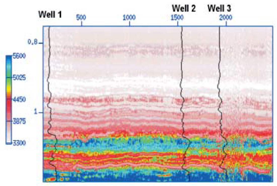
In our first test, only Well #2 was utilized to train the SVM. The resulting regressor was utilized to propagate the compressional velocity to lateral positions covering the complete seismic section. The result is portrayed in Figure 3. Notice that there is good agreement with the sonic velocities at Well #1 and Well #3. It is important to stress that these two boreholes were considered unseen during this test.

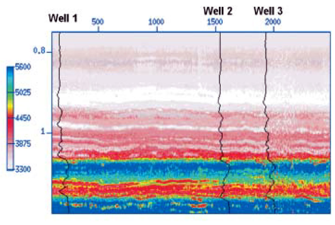
In the second test, we simultaneously trained the SVM with the three boreholes.

The resulting velocity model is displayed in Figure 4. In this case, the agreement with the know velocities at the borehole locations is quite remarkable.

Conclusions

A method to integrate borehole and seismic attributes was proposed. The method is based on the application of an unsupervised learning method, Support Vector Machine, to guide borehole-derived properties through a seismic volume. The system of equation arising during the learning stage of the SVM was solved using a Bayesian strategy. The latter provides a methodology for hyper-parameter selection, an important problem that has to be carefully addressed in order to avoid overfitting or underfitting the SVM during the learning stage.

Acknowledgements

We would like to acknowledge the following companies and agencies: Geo-X Ltd., EnCana Ltd., Veritas Geo-services, NSERC, and AERI (Alberta Energy Research Institute).