Seismic curvature attributes for mapping faults/fractures, and other stratigraphic features

Seismic attributes are a powerful aid to seismic interpretation, providing geoscientists with alternative images of faults and channels that can be used as components in unraveling the depositional environment structural deformation history. While seismic attributes have been used for nearly four decades, some of the most significant attribute developments and applications did not appear or gain acceptance until the pervasive use of 3D seismic technology in the early 1990s. Bahorich and Farmer’s, (1995) coherence attribute has become a common interpretation tool, being available in some form on most interpretation workstations. Curvature attributes were introduced in the mid 1990s as computed on horizon surfaces and shown to be highly correlated with fractures, some of them measured on outcrops (Lisle,1994; Roberts, 2001). More recently, volumetric curvature attributes have become popular, enabling interpreters to delineate small flexures, folds, mounds, and differential compaction features on horizons that have not been explicitly picked and that are otherwise continuous and not seen by coherence. In this article we discuss curvature attributes and some of their applications.

In a general sense, curvature is a measure of how deformed a surface is at a particular point. The more deformed the surface, the larger its curvature. By coupling such quantitative observations of structural deformation seen as flexures and folds along with more conventional images of faults, geoscientists can use well-established models of structural deformation coupled with well control, to predict paleostress and areas favorable to natural fractures. Curvature allows us to map stratigraphic features in addition to faults and fractures, as we shall describe here.

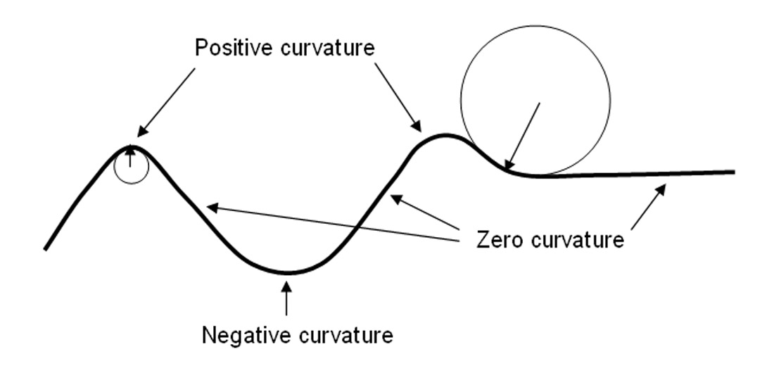
For a two-dimensional curve, curvature is defined as the reciprocal of the radius of a circle that is tangent to the given curve at a particular point (Figure 1). Curvature will be large for a curve that is tightly folded and will be zero for a straight line, whether horizontal or dipping. As a convention, anticlinal features are assigned a positive and synclinal surfaces a negative value.

This simple definition of curvature for a two-dimensional curve can be extended to a three-dimensional surface by imagining the surface being intersected by an orthogonal set of two vertical planes. This intersection describes curves on the surface for which curvature can be computed as we described in 2D above. Curvatures measured in planes perpendicular to the surface are called normal curvature s. Of this family of curves there exist two curves perpendicular to each other representing the maximum and minimum curvature. The maximum curvature is commonly used to map faults.

In actual practice, curvature is usually computed from picked horizon surfaces interpreted on 3D surface seismic data volumes by fitting mathematical quadratic surfaces on the surface patches of a given size. The actual curvature measures, including minimum, maximum, most-positive, most-negative, dip, and strike curvature, curvedness, azimuth of minimum curvature , and shape index are then computed from the coefficients of the quadratic surface. We find the most-positive and most-negative curvatures to be the easiest measures to visually correlate to features of geologic interest.

The interpretation of a seismic horizon may be a simple task if the quality of the seismic data is good and the horizon of interest corresponds to a prominent impedance contrast. Figure 2a shows a timestructure map at about 2000 ms interpreted from a 3D seismic volume acquired in Alberta, Canada. The horizon surface was manually picked in the form of a grid of control lines, followed by auto-tracking and application of a 3x3 mean filter to generate the horizon-based curvature images displayed in Figures 2b and d. Notice that both these displays are contaminated by strong acquisition footprint throughout with particularly strong footprint highlighted by yellow ellipses. Whether due to limitations in the survey design, coherent noise, or systematic errors in the processing, acquisition footprint is highly correlated to the source and receiver geometry and has little direct correlation to the subsurface geology. These types of overprints are artifacts and do not make any geologic sense. Horizons picked on noisy seismic data contaminated with acquisition footprint, or when picked through regions where no consistent impedance contrast exists (such as channels, turbidites, mass transport complexes, and karst), can lead to inferior curvature measures. One partial solution to noisy picks is to run a spatial filter over them, taking care to remove the noise, yet retain the geologic detail. Most commercial interpretation software provides a basic suite of such spatial digital filters.

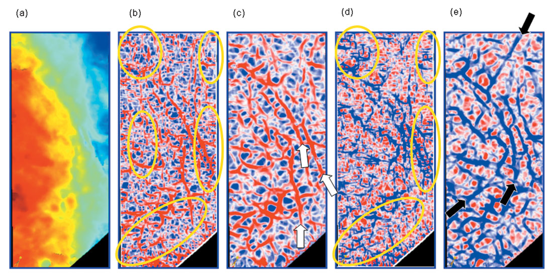
A significant advancement in the area of curvature attributes has been the volumetric estimation of curvature introduced by Al-Dossary and Marfurt (Geophysics, v.71, no.5, p41-51, 2006). This volumetric estimation of curvature alleviates the need for picking horizons in regions through which no continuous surface exists. In this article we report the results of our investigations into both horizon-based and volumetric curvature attribute applications. In spite of adopting spatial filtering, the horizon-based curvature estimates shown in Figures 2b and d still suffer from artifacts. In contrast, the most-positive and most-negative curvature attributes extracted along the extracted horizon surface in Figure 2a shown in Figures 2c and e are free of these footprint artifacts.

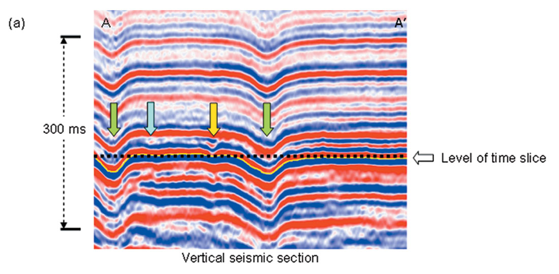
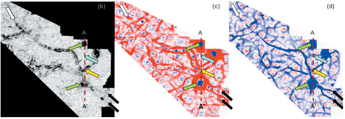
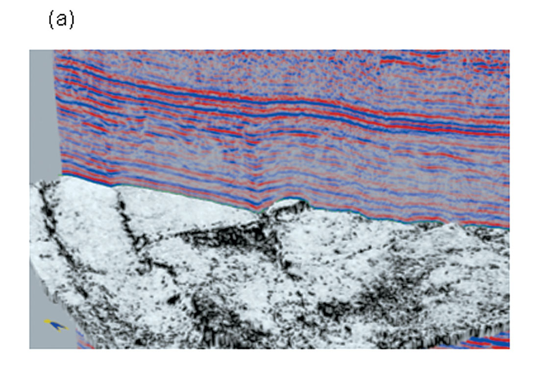
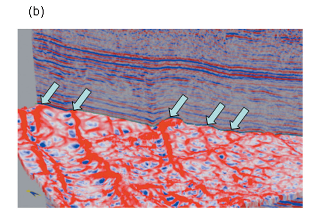
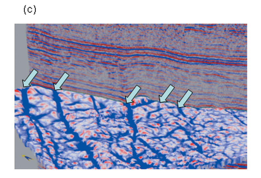
In Figure 3 we display display time slices through volumetric estimates of coherence, most-positive and most-negative curvature. Notice the clarity with which the main NW-SE channel (black and white block arrows) stands out, in addition to the 3 prominent collapse features. A second channel system appears in the northeast corner of the image and intersects the main channel half-way. The most-positive curvature defines the flanks of the channels and potential levees and overbank deposits, while because of differential compaction the most-negative curvature highlights the channel axis or thalweg. The coherence image is complementary and is insensitive to structural deformation of the surface; rather it highlights those areas of the channel flanks where we have a lateral change in the waveform due to tuning. In Figure 4 we show the correlation of the attribute time slices with the seismic sections, an exercise interpreters need to go through to understand and visually validate how the attribute features match the seismic signatures. Again, the definition of the channels (edges and thalwegs) is seen clearly on both the most-positive and most-negative curvature displays in preference to coherence.

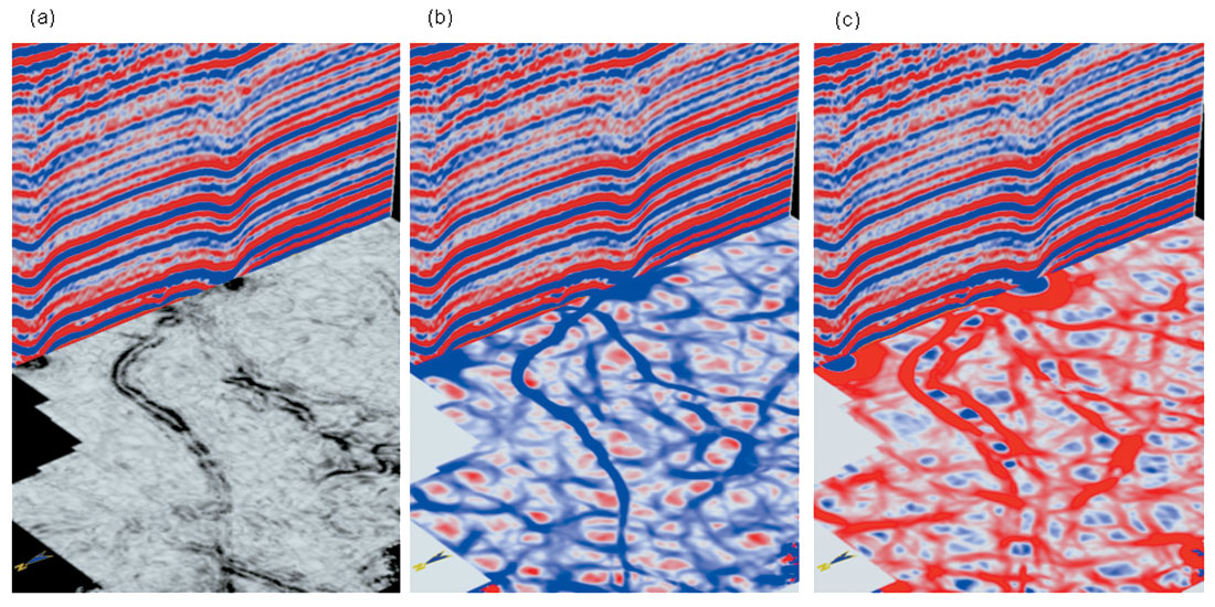
The value of volumetric attributes is two-fold. First, as shown in Figure 2 (and more in Figures 3 and 4), the images have a higher signal-to-noise ratio than horizon-based attributes. Volumetric estimates of curvature are computed not from one picked sample, but rather from a vertical window of seismic samples (in our case, 11 samples), such that they are statistically less sensitive to backscattered noise. Second, not every geologic feature that we wish to interpret falls along a horizon that can be interpreted, such as the channels shown here.

Coherence is an excellent tool in mapping faults represented by discrete reflector offsets. Unfortunately, most seismic data volumes are imperfectly imaged. Errors in static corrections, velocity analysis, and the use of time migration rather than depth migration may result in smeared images of faults that may otherwise exhibit discrete reflector offsets. Imbricated faults, faults with sediment drag along them, and faults whose offset is a fraction of a wavelet will not be imaged well by coherence. Curvature sees such faults as ‘flexures’.

Curvature displays are particularly helpful in bringing out the definition of subtle faults and fractures that may help in the placement of horizontal wells. In Figure 5 we show chair displays of strat-cubes (A strat-cube is a sub-volume of seismic data or its attributes, either parallel to a picked horizon or proportionally sliced between two non-parallel horizons) from coherence, most-positive and most-negative curvature volumes intersecting a seismic line that cuts the fault/fracture trends orthogonally from a 3D seismic volume from the Middle East. Notice, how the red peaks (Figure 5b) on fault lineaments (running almost north-south) correlate with the upthrown signature on the seismic. Similarly, the most-negative curvature strat-slice intersecting with the random seismic line (Figure 5c) shows the downthrown edges on both sides of the faults highlighted in blue.

Curvature attributes for well-log calibration

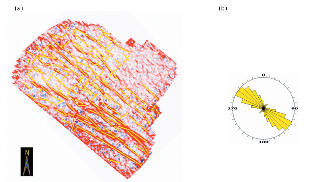
Figure 6a shows a horizon slice extracted from a most-positive curvature volume at an appropriate level in the zone-of-interest. There are a number of fault/fracture lineaments, which we have tracked in yellow. We then combine the density and orientations of these lineaments in the form of the rose diagram shown in Figure 6b, retaining the color of the lineaments. This rose diagram can be compared with a similar diagram obtained from the image logs to gain confidence in calibration. Once a favorable match is obtained, the interpretation of fault/fracture orientations and the thicknesses over which they predominate can be trusted for a more quantitative analysis, which in turn could prove useful for production from compartmentalized reservoirs.

Conclusions

Like all attributes, curvature is valuable only when coupled with a geologic model of structural deformation, stratigraphic deposition, or diagenetic alteration. Curvature is particularly sensitive to flexures and faults. Curvature can be a powerful tool in mapping channels, levees, bars, contourites, and other stratigraphic features, particularly in older rocks that have undergone differential compaction such as the examples shown here.

Discrete fractures often appear on most negative curvature, though the cause can be either due to sags about the fractures or due to local velocity changes associated with stress, porosity, diagenetic alteration, or fluid charge. Although curvature attributes run on time surfaces after spatial filtering can often provide valuable results, volumetric curvature attributes provide valuable information on fracture orientation and density in zones where seismic horizons are not trackable. The orientations of the fault/fracture lineaments interpreted on curvature displays can be combined in the form of rose diagrams, which in turn can be compared with similar diagrams obtained from image logs to gain confidence in calibration.

Acknowledgements

We thank Arcis Corporation and Olympic Seismic, Calgary for permission to show the data examples and Arcis Corporation, Calgary to publish this work.