Useful Mistakes, Cognitive Biases and Seismic

We come to conventions and Symposia to hear about success and bask in the glory of our awesome, successful colleagues. But mistakes may also lead to useful learning opportunities. After all, we often mistakenly look upon our successes as if they are the result of some intrinsic property of ourselves, as if we are both special and right, rather than consider that at least some of them have come about their success due to luck. A failure or an error, on the other hand, may be far more illuminating and attention holding if we allow ourselves to honestly face up to it.

I was humbled and grateful to have been chosen as the Honoree at this year’s CSEG Symposium. As has been customary in past Symposia, a group of very intelligent people did make a heroic effort to say some nice things about me. Looking back on my own career, I do see some things that I am proud of. I see a great many people who I am proud to have worked with. Scott Reynolds spoke of some of those excellent people in his Tribute talk, which I hope will be published. I see a few problems (sort of) solved and situations improved. All that is wonderful, but my career trajectory looks the way it does because I had a great many things to learn. I made errors. I was part of some mistakes. I was the ringleader of a few of them. My work suffered from a variety of cognitive biases, and many of the very intelligent people around me did as well. In the second half of my time as a geophysicist, I became more aware of some of my faults, errors, and shortcomings. I attempted to become a better scientist and make less cognitive errors. It turns out that both tasks are difficult.

This write up of some of the elements of the talk I gave at the Symposium delves into certain mistakes I made or was a part of and discusses why they were made. In fact, the systemic reasons for the mistakes are far more important than the mistakes themselves. It is unlikely that future geoscientists will find themselves in the identical situations that I have erred in, but they will, like me, be human.

It’s not just me: ask the military

In speaking of my own mistakes, I am neither attempting to humble-brag or to suggest that I was an awful geophysicist. It is more likely that I was generally typical but had an unusual tendency to communicate about my work. Certainly, I worked with an excellent group of professionals. Everyone—myself, my peers, partners, cross-disciplinary colleagues—wanted to do a good job, keep costs and environmental impacts low and bring in a high return on investment for our employers. None of us wanted to make mistakes. But we did. Lots of them, many of which slipped by without us even realizing it. Most of our errors were never covered in a university geosciences or physics course, in company training or in any technical conference. Most of our errors, the ones that we committed again and again were as a result of the human condition, because of the biases and limitations that human beings tend to have.

In his book, Men Against Fire, Marshall (1947) discusses at length the fact that over 70 percent of all infantry soldiers do not fire their weapons in actual combat, even if the vast majority will fire in combat exercises or on the firing range. Marshall quite adroitly realizes that to address this issue, the feelings, or the morale of the soldiers must be addressed. While Marshall appears loathe to use the vocabulary of the psychologist, it is inescapably the feelings and biases of the soldiers that are his main points of enquiry in the book. Without uncovering the psychological reasons for the inability of most soldiers to follow the most basic and essential order they can receive, there can be no improvement in performance. And so it is for geoscientists. While we are in no way driven to the farthest extreme of action or mortality in our jobs, we nevertheless are human beings who are subject to common pressures, common cognitive biases and make common, systemic mistakes.

Psychology, there is a better goal than to manipulate others to our ends

The study of human behavior is a ubiquitous tool of the modern world. Nobel prize winner Richard Thaler’s nudge theory is at work in most modern choice tests. Nudge theory (Thaler and Sunstein, 2008) influences behavior using subtle methods such as the careful selection of the default choice on medical tests, municipal polls or dietary questions. Politicians, salesmen and marketers use the nudge theory; it affects us daily as our decisions on buying and policy as it is pushed by one actor or another. Users of the theory claim they are doing it for our own good, though we can only guarantee that the theory is used to influence us for theirs’. Daniel Kahneman is another Nobel prize winner who wrote Thinking Fast and Slow (2011), an expansive summary of his studies of cognitive biases that has been hugely influential in economics. There are few policy makers or professional marketers who are unaware of the work of Kahneman and the behavioral psychologists. The use of such knowledge of humanity makes sense. If we want to influence how others buy, think or vote—how they choose—we should understand how they think, buy and vote.

Behavioral psychology seems to be used most in practice to manipulate or influence others. It does not matter that some who do so, do it in the name of beneficent sounding terms such as libertarian paternalism, it is still a tool being applied by others onto us. But if the tools of psychology are useful for others to attempt to influence us to better choices, why do we not attempt to use our knowledge of psychology to help ourselves make better decisions? Better geoscientific decisions? An inward use of the knowledge certainly has the advantage of being used towards benefits that we choose.

But how can we do this? The answer to this question brings us back to my mistakes. My mistakes are useful because they can be used as an example to bridge the gap between some of the lessons of behavioral psychology and the choices made by geoscientists.

Maslow’s Hammer and Experimenter’s bias

Maslow (1966) said the now famous, “[To a hammer, everything is a nail].” He was speaking of the extraordinarily strong tendency of human beings to rely—sometimes to their detriment—on familiar, comfortable tools, whether they are appropriate or not to the problem at hand. This cognitive bias has many names that can be used to impress friends at parties. The law of the instrument, the Birmingham screwdriver, the golden hammer, or the Einstellung Effect are just a few. Geoscientists are no exception to this human tendency to use what we are used to, what we are well versed with, or with what has perhaps gotten us notoriety or economic success in the past.

Even if we may forgive ourselves for depending too much on Maslow’s Hammer, we geoscientists are likely less comfortable when considering our own use of experimenter’s bias. Jeng (2006) makes a survey of this bias, which is our predilection to believe, publish and promote data that agrees with our expectations and to ignore, suppress or denigrate data that conflicts with those expectations. Maslow’s Hammer likely plays a part in this bias, for preferred outcomes—or expectations—will often go hand in hand with a preferred tool. Experimenter’s bias is the more uncomfortable bias because it contradicts our feelings of scientific integrity. And yet we may ask, how many examples of failure do we see in the literature of the CSEG?

Example one: the frustratingly non-unique Radon transform

The Radon transform went through a period of great and manifold development for seismic applications starting in 1985, lasting for about twenty years. This development is remarkable for its ingenuity alone but is also noteworthy because the problem of experimental bias played an ongoing role.

The Radon transform essentially represents data in time and space by families of curves with onset times (tau) and ray parameters (p). The hyperbolic family was identified early on as being apt for separating primary and multiple events of common midpoint gathers (CMP) by creating a velocity space. Unfortunately, there are several well-known mathematical issues with the Radon transform, chiefly its ill-posedness. Thorsen and Claerbout (1985) discussed how the ill-posedness of the transform is exasperated in seismic by missing data in the CMP gather, chiefly at the near offset and far offset. The data truncation at these edges can never be fully removed in seismic data—such would be physically impossible—and it creates a smeared, non-unique response that limits the ability for primaries and multiples to be separated. To reduce the non-uniqueness of their results, Thorsen and Claerbout introduced sparsity constraints which reduced the smear in p space, though at horrendous—and at the time, potentially bankrupting—computational cost.

As a problem in logic, I will argue that no constraint, or inserted prior knowledge, can be truly effective if the physical assumption that it represents is not valid. That is, if the assumption is not true, the product of its use may be false. The sparsity constraints for the Radon transform are partially valid. The idea of the constrained transform simulating a gather of infinite offset range, and thus creating sparsity in p space makes intuitive sense, is easy to imagine, and was developed commercially in a series of steps. Hampson (1986) employed an ingenious method to make the transform work given the processing limitations of the time, though he was forced to give up on Thorsen’s sparsity and had to use parabolas instead of hyperbolas. Sacchi and Ulrych (1995) introduced a fast method for including sparsity in p, and Cary (1998) argued that only by including constraints in both tau and p can the necessary and sufficient conditions (Hughes et al., 2010) be met for a desirable solution. Cary’s explicit and correct use of logic is rare in the literature. Many others, including myself (Hunt et al, 1996) through to Ng and Perz (2004) illustrated the improved results of their sparse Radon transforms which were developed using these ideas.

Virtually all of these many papers—and most major seismic processing companies of the time seemed compelled to publish their own solution—showed near perfect synthetic results in which non-uniqueness was apparently eliminated. It is within these many papers and their near perfect, unique, synthetic results, that experimental bias was at work. Consider Ng and Perz’s (2004) paper and a redisplay of their Figures 1, 2a and 5a, below, which I rename Figure 1. We see in Figure 1a the input CMP, which is moveout corrected and has only one primary of tau 1100ms. The rest of the events, including another event with tau of 1100ms, are multiples. Figure 1b shows the non-sparse Hampson (1986) algorithm’s Radon transform space. It shows the smeared truncation artefacts and some overlap of energy in p at a tau of 1100ms from the primary and multiple. Figure 1c shows Ng and Perz’s (2004) sparse Radon algorithm’s space. Events are well localized in tau and p. The two events at a tau of 1100ms are distinct and separate.

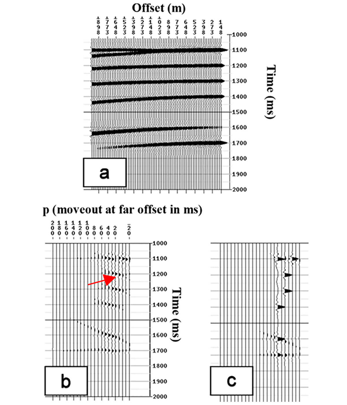
This example is typical of the many papers of the time and makes the argument that these sparse algorithms have virtually eliminated the non-uniqueness in the Radon transform. No author that I am aware of has claimed to have completely eliminated non-uniqueness, but the examples given show positive synthetic results with no material uniqueness issues remaining. A reader of such papers likely knows that the sparsity will eventually fail to mitigate the non-uniqueness at some tiny moveout (the authors certainly know this), but these examples are generally not shown. This omission by itself is an argument for experimental bias, but the bias is in fact much more overt.

Hunt et al (2011) showed that there are other relevant variables impacting both the effectiveness of multiple attenuation and the uniqueness of the Radon transform. Yes, I had historically been an unwitting part of the experimental bias, but this further examination into the problem of short period multiple elimination made myself and my co-authors (who included Mike Perz from the 2004 paper) realize that this cognitive bias was denying us a better understanding of the non-uniqueness problem in the Radon transform and in its use for effective multiple attenuation.

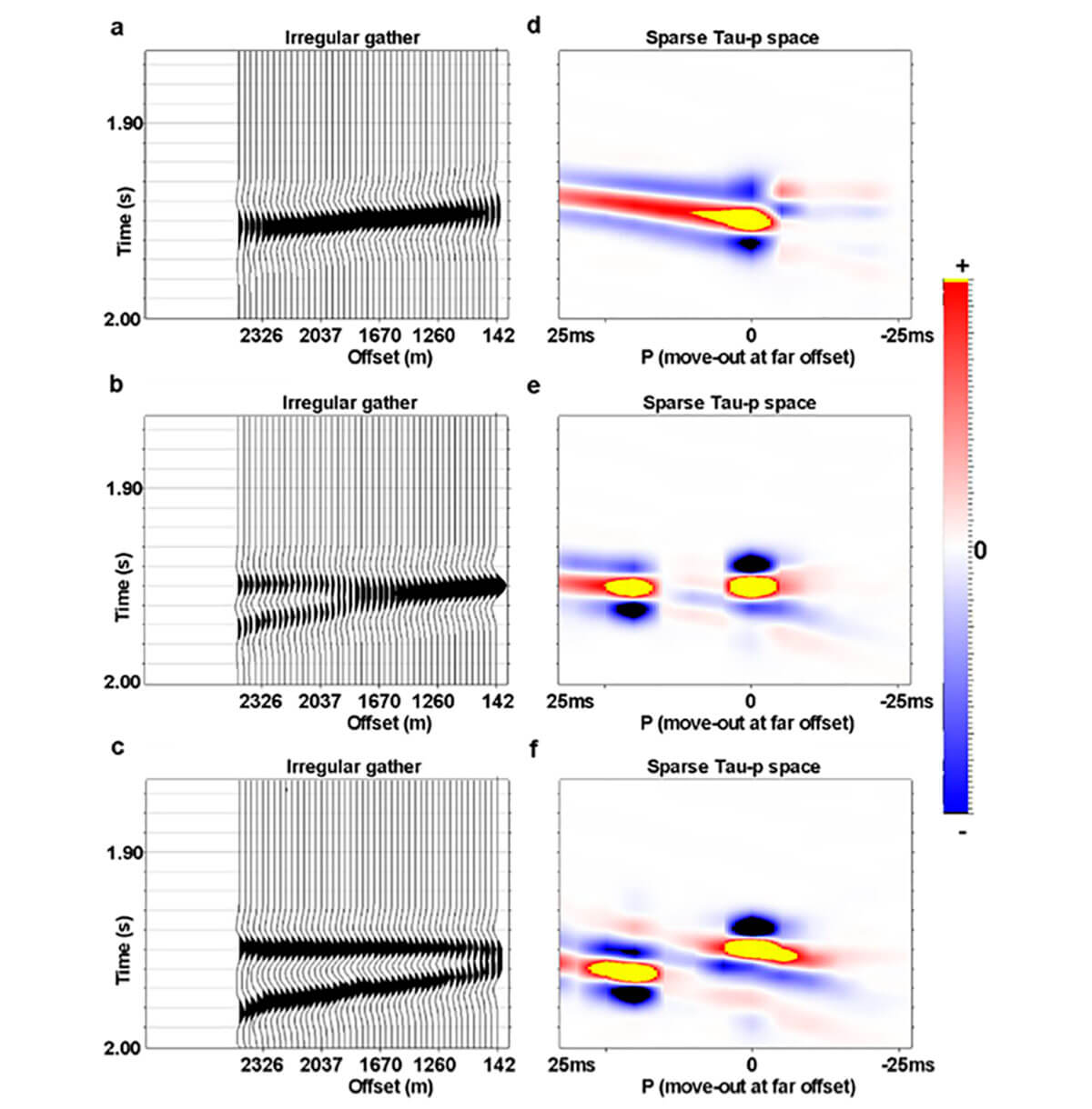
Figure 2, from Hunt et al (2011) shows an example of non-uniqueness in the Radon transform space due to varying onset, or tau, times of primary and multiple events. Figure 2 illustrates a primary and multiple with the same amplitudes. The differential move-out of the multiple with respect to the primary is 20ms at 2500m offset. The intercept time, Tau, of the multiple is varied and the offsets were taken from a typical CMP from the 3D to simulate land 3D irregularity. A 35 Hz Ricker wavelet was used for each element of this figure. In Figure 2a, the multiple starts 10ms above the primary, in Figure 2b both events start at the same time, and in Figure 2c, the intercept of the multiple is 10ms below the primary. The corresponding sparse Radon transform spaces are shown in Figures 2d, 2e and 2f. The primary and multiple are not resolved in Figure 2d. In Figure 2e, two events are resolved in p, but the position of the multiple is slightly incorrect. Only in Figure 2f are the primary and multiple separately resolved and in their correct positions. Relative onset times by themselves control tuned character on the CMP gathers, which unsurprisingly controls uniqueness in the Radon transform space of even sparse algorithms. This is a material observation of the transform’s continuing non-uniqueness. How was this missed from the literature except by experimental bias?

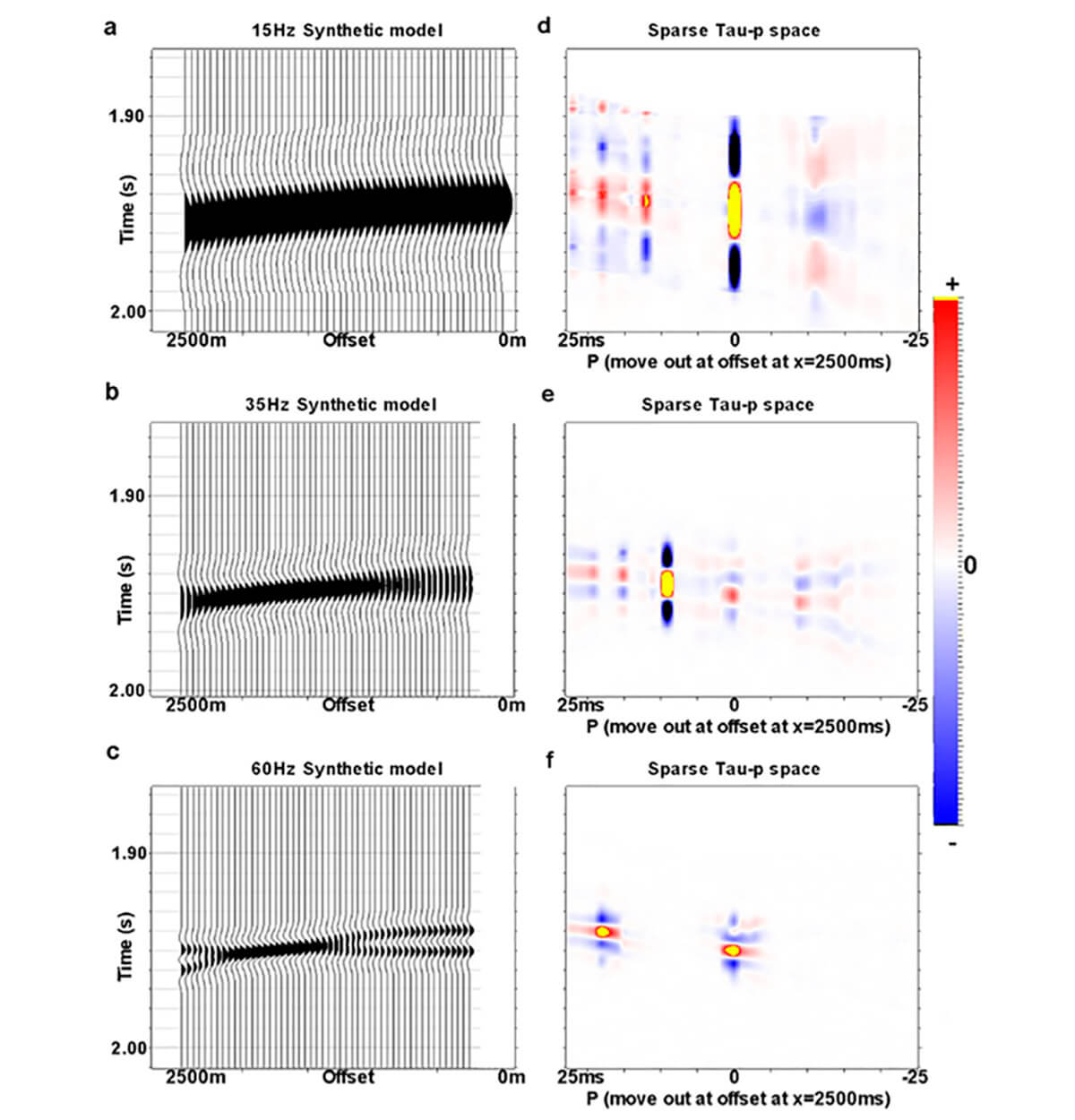
Let us examine the effect of changes in wavelet size on the ability of the sparse Radon transform to separate multiples and primaries properly (Hunt et al, 2011). The simple model of Figure 3 illustrates this effect. A primary and multiple are depicted in Figures 3a, 3b, and 3c. In each case, the multiple starts 10ms above the primary, and has a differential move out of 20ms at 2500m. The primary and the multiple have equal amplitude, and the offset bins are perfectly regular. The only differences in these three images are that the wavelet of the data changes from a 15 Hz Ricker in Figure 3a, to 35 Hz Ricker in Figure 3b, to 60 Hz Ricker in Figure 3c. Figures 3d, 3e, and 3f, represent the sparse Radon transform spaces for Figures 3a, 3b, 3c, respectively. The Radon transform space corresponding to the low resolution gather of Figure 3d clearly does not resolve the primary or the multiple; most of the energy is on the zero moveout curvature. The mid resolution gather fairs little better: Figure 3e shows the energy is misallocated in quantity and position. Only the highest resolution gather of Figure 3c and its Tau-p space of Figure 3f does a perfect job of resolving both events, and correctly representing the move out of each event. The greater the wavelet resolution, the less non-uniqueness in the Radon transform. That resolution affects the uniqueness of the Radon transform should have been obvious, but it had not been a focus of the work to this point. By explicitly illustrating this now unsurprising shortcoming, Hunt et al (2011) were able to focus on increasing the resolution of the wavelet as much as possible.

What are we to glean from this example? I had been a small part of the history of experimental bias concerning the non-uniqueness of the Radon transform. This cognitive bias was not at work as part of a conspiracy. The authors were honestly attempting to reduce non-uniqueness in the transform. But that these two obvious sources of non-uniqueness were never explicitly shown in the literature until recently suggests that experimenter’s bias exists. We rarely show the bad examples or look for them. We human beings are caught focussing on the narrow little points of our main purpose and we toss aside—often unthinkingly—that which does not contribute to that simple coherent idea. Some readers will note the coherency bias (Kahneman, 2011) at this point. In the case of the Radon transform, there is little doubt that the authors involved did improve the non-uniqueness of it. But they missed an opportunity to do a better job and gain a clearer understanding by not highlighting these limitations.

Example two, experimental bias and Maslow’s Hammer with AVO

Amplitude versus offset analysis (AVO) is one of the most popular diagnostic tools of the modern seismic practitioner. It enables elastic rock property estimates of the earth from a large portion of the historical p-wave seismic data. As useful as AVO derived estimates can sometimes be, geophysicists may sometimes come to over-rely on them and may also sometimes apply experimenter’s bias where they are concerned.

In the 2012 CSEG Symposium, I showed a case study regarding the controls on Wilrich production where AVO was shown to be ineffective. The most pressing questions from the audience were not on the many details of the novel method that I and my co-authors had created to quantitatively demonstrate the importance of steering to obtain better productivity but were instead obsessed on why I could not make AVO “work”. When my coauthors and I later published this study in Interpretation (Hunt et al, 2014), the biggest questions from the peer-review again ignored the core work of the paper and focused on the apparent failure of AVO. I was told that I had to prove why I did not include AVO estimates in my method. This is quite apparently an example of both experimenter’s bias and Maslow’s Hammer.

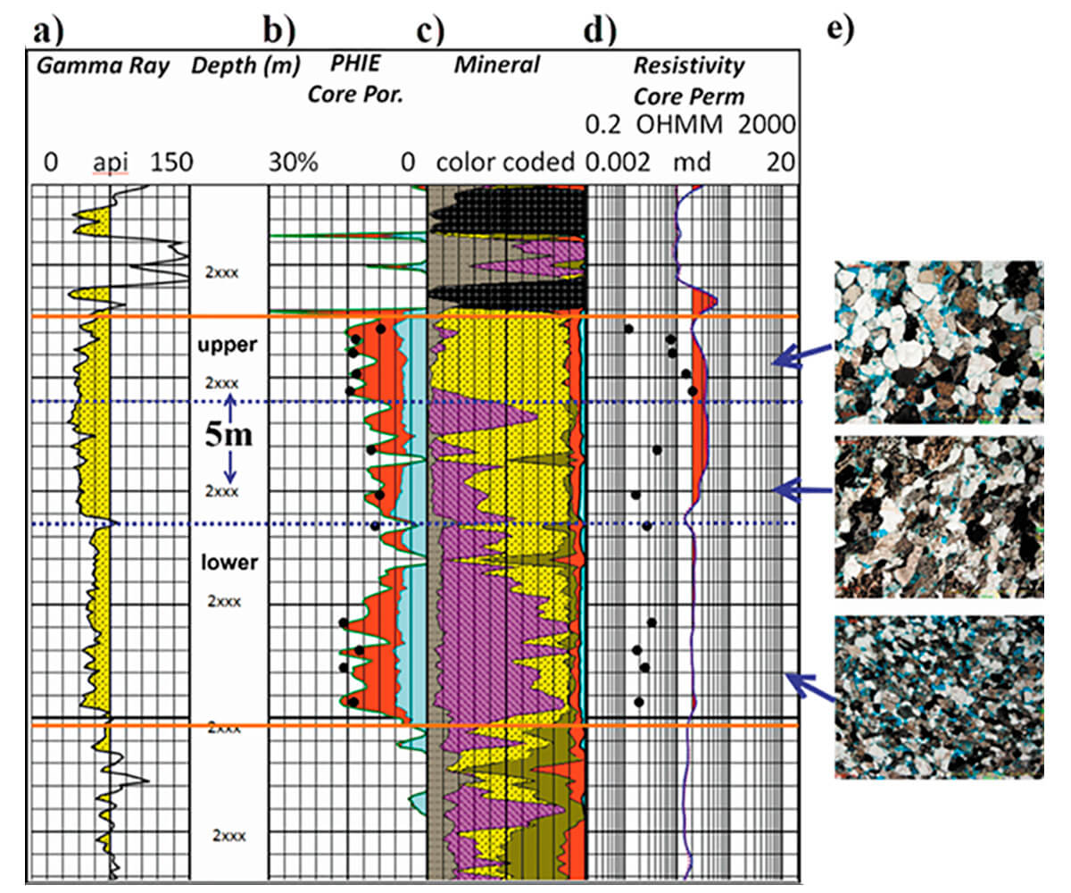
The target the work was the tight, deep basin, Wilrich sandstone in Alberta Canada, which exhibits low permeability (0.05 to 0.1mD) and low to moderate porosity (6% to 8%). Figure 4 is the petrophysical type log used in the paper. The agreement of log effective porosities is shown in Figure 4b, the mineralogic content is shown in Figure 4c. The core effective permeabilities of Figure 4d and the thin section images of Figure 4e were important elements of the paper which was concerned with how well each of the upper, middle and lower section of the Wilrich would contribute to production and if relative well placement in a particular zone would be important. Of importance is the coal section, shown in black shading in Figure 4c, which lies directly on top of the Wilrich sand. This coal section is of variable thickness in the area and has materially different rock properties than the Wilrich.

Hunt et al (2014) evaluated well length, fracture stimulation data, geologically mapped porosity thickness (Phi-h), reservoir pressure, mud gas and gamma ray logs, relative position of the horizontal wellbore in each of the upper, middle, and lower Wilrich as estimated quantitatively from wellsite data. To this was added interpreted 3D seismic data including stack response, AVO (including inverted Lame parameters), azimuthal AVO (AVAz), velocity variation with azimuth (VVAz), curvature and coherency in an exhaustive array of windows about the Wilrich. All these parameters were gridded along the horizontal wellbores and made correlatable to each other as well as to productivity on a wellbore by wellbore basis. Using the seismic to estimate bin by bin seismic Phi-h estimates along the wellbores was highly desirable, so an exhaustive effort was made to determine if any of the seismic variables, chiefly stack and AVO or AVO inversion variables would correlate to the 114 vertical control wells, each of which had an effective Phi-h value from multimineral geologic well analysis.

The effort to correlate seismic variables (including AVO) to the Phi-h of the vertical wells failed completely and was the only exigent issue to audience members at both the Symposium in 2012 and to the peer review process in Hunt et al (2014). The questioning of this failure was remarkable in a paper in which AVO was but one tool of many, and in which production estimation, not AVO estimation was the key scientific question. Having been there, I can tell you that no one wanted AVO to fail. I know this because of the direct communication made to me as first author, and because I also wanted AVO to be effective. This experience was a searing example of experimenter’s bias. Hunt et al (2014) did exhaustively prove, through modeling and real data correlations, that AVO both could not and did not predict the Wilrich Phi-h. They also proved why. It was because of the variable overlying coal, which directly overlay the sand, and which dominated the reflection response at all angles of incidence.

All but ignored in the angst over the failure of AVO to be effective in the estimation of the Wilrich sand Phi-h, were several important lessons. Figure 5 shows the correlation coefficients for a few of the seismic variables in the study as they related to both Wilrich sand Phi-h and the overlying coal isopach in the 114 vertical wells. None of the seismic attributes passed the 1% p-test of statistical significance for predicting the Wilrich Phi-h. All but one (the curvature) of the seismic variables had a statistically significant correlation to the coal isopach.

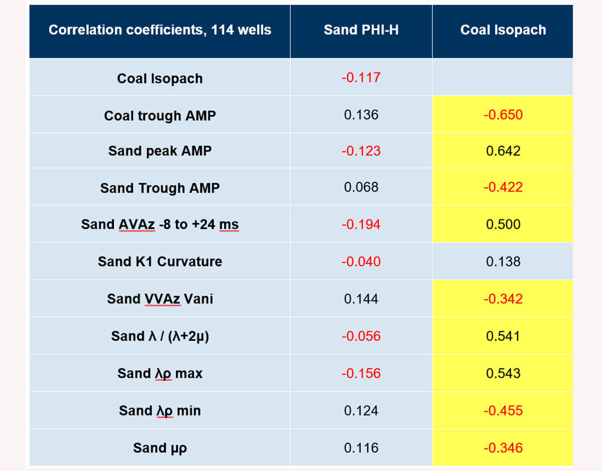
The key lessons here are manifold:

1. The seismic attributes were ineffective for predicting Wilrich Phi-h, but this is not necessarily because they did not “work”. The opposite is likely true.
2. The seismic attributes, including AVO and AVAz, were correlated to the coal isopach. This is because these attributes are reflectivity based. AVO did likely work, just not in a way that was useful to the commercial purpose at hand.
3. That AVAz response is reflectivity based is well known, but that it may be controlled by overlying coal, which is known to be anisotropic, is an important and obvious conclusion from this work.

Lessons #2 and #3, while not necessarily pleasing, were later repeated numerous times in other work that I engaged in, most of which was unpublished, except for the 2016 CSEG Symposium where Bahaa Beshry spoke of our stress work. There he showed again that AVAz measures showed statistically significant correlations to coal isopach in sections of the data where coal tuning is present. The biggest lesson here is that experimental bias can be so strong that we miss an unexpected but important learning.

Loss Aversion and Neglect of Probabilities, or when we are facing a loss, we often make it worse

The most common errors that I have been a part of have been caused by loss aversion and neglect of probability. For most of my career, I lacked the vocabulary to effectively treat this issue. Kahneman (2011) does an excellent job of illustrating these issues, which often go together, and providing language around these important cognitive issues. Loss aversion, simply put, is the irrational hatred that human beings have of taking a loss. This is not a suggestion that people should enjoy losing, but an observation of the objective fact that they dislike losing more than is rational. An example from Kahneman (2011) follows:

Which do you choose:
Lose $900 for sure or choose a 90% chance of losing $1100?

Kahneman studied this and many similar questions empirically and found that the choice most people make is to take the gamble, which is laughably irrational. Kahneman’s conclusion is that when all options are bad, people like to gamble.

Note that the expected value of each decision is the matter of simple arithmetic. It may be that some of those who chose the gamble had performed this arithmetic and knew that the gamble had a larger expected loss, but it is likely that many did not even extend their effort even to this trivial level. In the world of geosciences and business operations, matters often go wrong, and similar—though more complex—choices will arise. The probabilities and expected values relevant to such choices may not be so glaringly obvious. Geoscientists and decision makers often have another meta-choice before them: to gamble blindly or lay out the probabilities and expectations in a rational decision-making framework.

The most vexing observation from my experience is how often, in a business with ubiquitous uncertainty, that we have disregarded probabilities when make decisions. This is common cognitive bias is called neglect of probability. It appears to go hand in hand with loss aversion, and often exacerbates it.

We might deny that we have made irrational decisions due to loss aversion and neglect of probabilities, but there is seldom a signpost or adjudicator that stops us and tells us when this is happening. I have observed or been an active participant in these biases at many of the companies that I have worked at. On some occasions, I have suspected that our decision processes have been in error but have lacked the vocabulary or tools to properly address the issue. Sometimes, I am sure, that the other decision makers have also suspected that irrational choices were being made. Some of the general circumstances in which these biases have occurred are:

• Following a property acquisition, and we discover we paid too much, so we have acted rashly, hoping to “drill our way out” of the mistake and avoid facing the loss.
• After operational issues with drilling, when significant money has been spent and we face an attempt to remediate the operation or abandon it. Choices are often made with an irrational bias towards further operations in the original wellbore.
• After completion issues in a new operation, and we face the loss of the wellbore.
• Every time we fail to quantitatively determine the predictive accuracy of our seismic attributes / data / interpretation to the target property under which a decision is about to be made.

Virtually every element of geoscientific advice we give has an element of uncertainty to it, and if we do not in some way address this, we may be engaging in neglect of probability.

Example three, operations and Loss Aversion and Neglect of Probabilities

At one of my companies, we drilled a long, deep, expensive horizontal well. Wellsite data was incredibly positive, and we were quite certain that the wellbore would be highly economic. The open hole completion equipment was placed, but the wellbore abruptly failed within the near-heel portion of the horizontal section.

The decision at hand was whether we should attempt to remediate the wellbore or to drill an entirely new well (a twin), which would cause us to take a multi-million dollar loss on the first (failed, under that decision) well. In the multidisciplinary meeting where this decision was taken up, the initial feeling was that the remediation choice would be best.

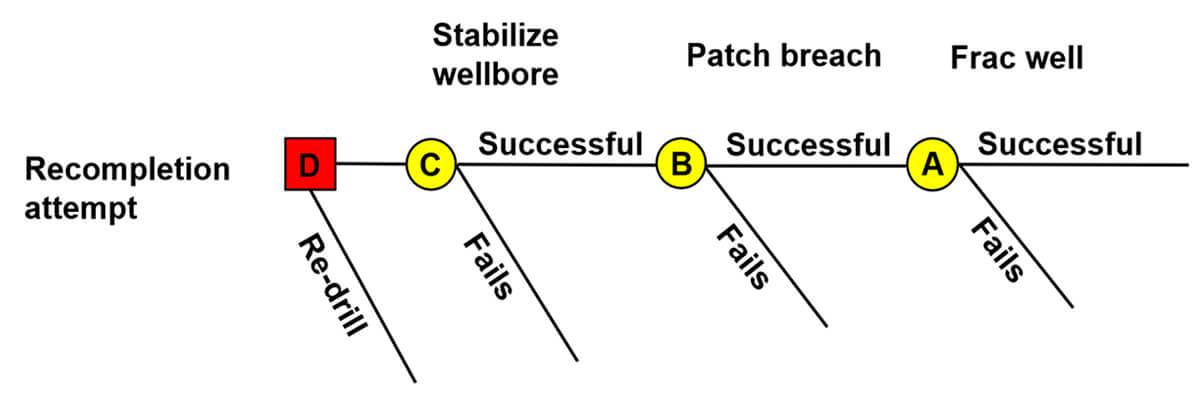
But I had seen this type of issue before, and it was suggested that we consider the problem using decision analysis (Newendorp, 1975), create a decision tree, and populate it with the correct probabilities and costs. Figure 6 shows the cartoon decision tree. To successfully remediate the original well, three operations had to be successfully executed: the stabilization of the wellbore, the patching of the breach, and the subsequent fracture stimulation of the well. The decision analysis was quite simple, and its construction was not time consuming, nor were the probabilities difficult to populate by the operational team. The analysis clearly showed that, in this example, the remediation path had a lower expected value. The decision to twin was made, and the twin was successful. The cumulative effect of considering the three sub-probabilities of the operation yielded a much different, and easily measurable answer than when considering the operation as a whole.

A world with no mistakes

The only productive reason to review mistakes, or decisions made under cognitive biases, is to improve our decision making going forward. An understanding of logic and behavioral psychology is neither best put towards conceits at a cocktail party nor to manipulating others. This knowledge is best applied inward, to improve ourselves and our decision processes. This is not something to learn once and feel superior over, it is a thing to learn and relearn and be ever watchful of the moment when, ego-depleted or in a hurry, we forget the lesson and make a new mistake. To err is human, and to be human is to always have a set of error tendencies just waiting for the proud, lazy moment and our undoing.

We will never be free of fallibility in our thinking, or of potential biases.

While we may no more eliminate mistakes than we can eliminate our own humanity, we can on a case by case basis minimize them through awareness, wariness, and humility.