3-D Acquisition requires careful planning. Laying out lines of receivers and lines of shots must be done with an eye to the expected results. Computer programs are now available to assist the geophysicist in this task.
In this paper I shall discuss the general guidelines for designing 3-D surveys, and illustrate the methods with various examples.
Some popular 3-D Layout Strategies
In Figures 1 through Figure 7, we show some of the layout strategies most commonly used at the present time.
The straight line method is the easiest to layout in practice. It can accommodate extra equipment (layout ahead of shooting) and roll-along operation. All shots between adjacent receiver lines are fired, the receiver patch is rolled over one line and the process repeated.
In Figure 2, we see a variation of the straight line method. In swath shooting all shots between receiver lines that are several lines apart are fired. The receiver patch is rolled over several lines and the process repeated. The operational advantages are attractive, but the resulting offset/azimuth mix and the statics coupling are quite poor.
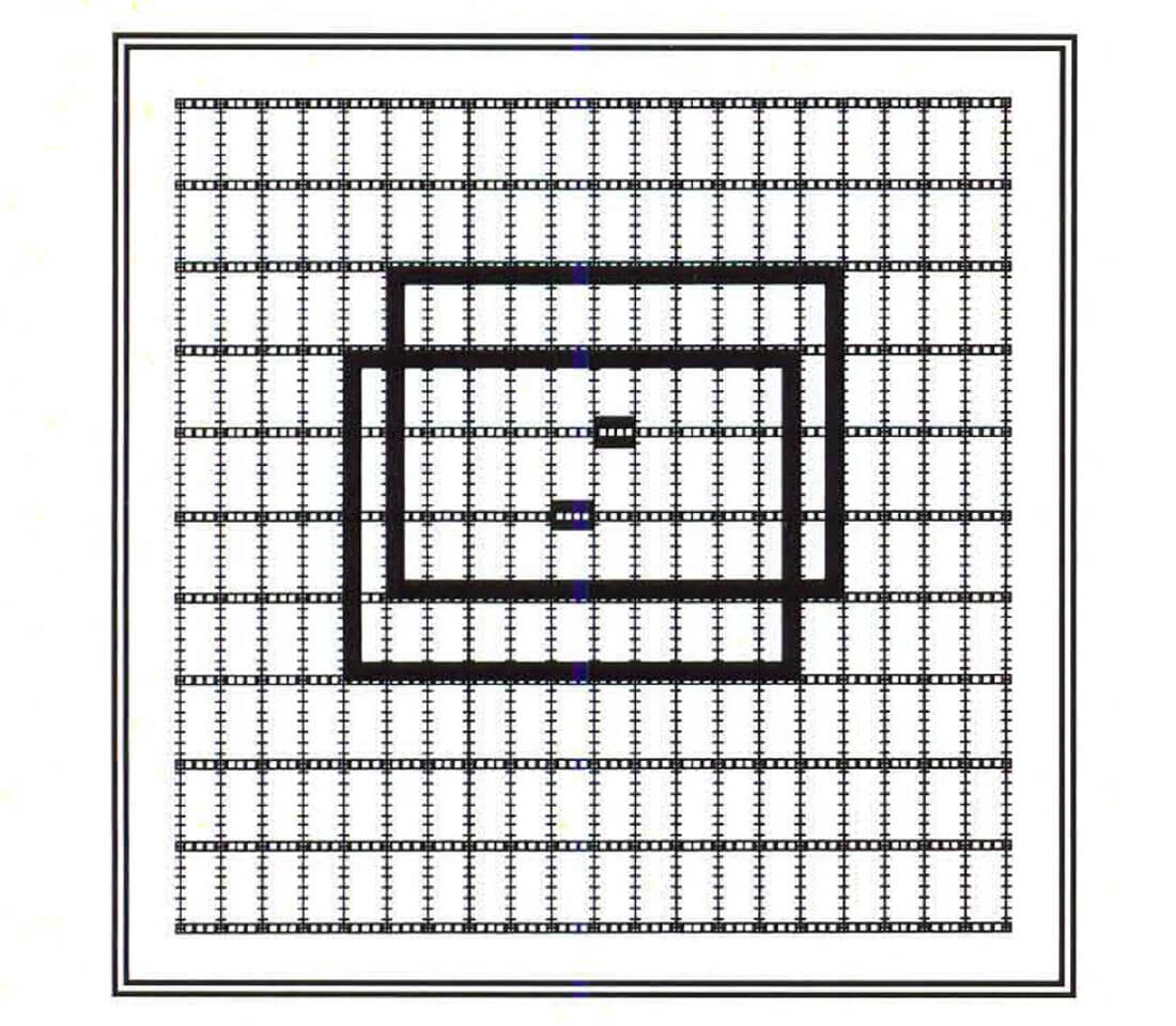
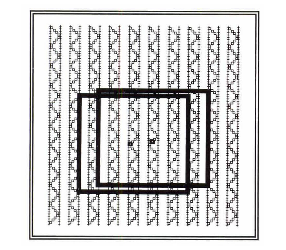
The Brick pattern shown in Figure 3 has one overwhelming advantage. If you consider a typical "Box" (the area between two adjacent shot and receiver lines and the smallest repeatable element of a 3D survey), then it should be apparent that the largest minimum offset will be equal to the receiver line interval (or shot line interval if this is smaller). In contrast, the Straight Line method in Figure 1 above, will have a largest minimum offset equal to the diagonal of one "box".This means we can increase the receiver line interval with this method, still retain the required minimum offset and save on costs. Access to shot locations is a potential problem with this method.
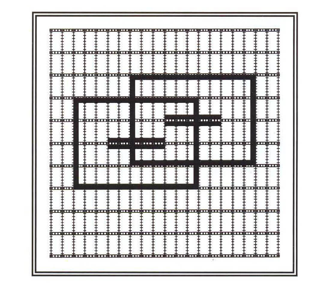
Odds and Evens shown in Figure 4 is really a variation on the Brick pattern. In this case there is a new "brick" every shot. Operationally you must traverse twice as many shot lines as the Straight Line method - but, of course, you only fire every second shot on each line. Statics coupling is weak in this method – for wavelengths equal to the inline shot interval.
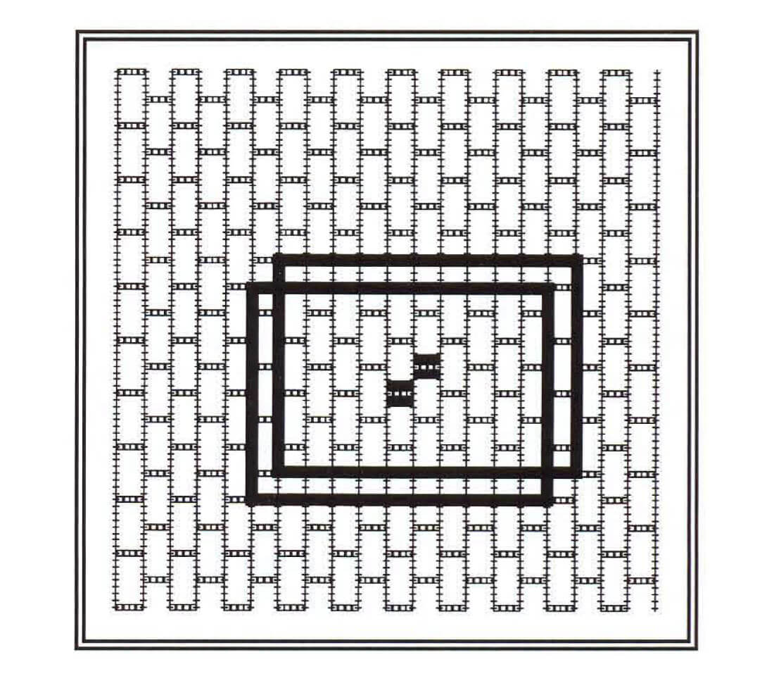
The Zig Zag pattern in Figure 5 is very popular in desert areas, or anywhere you can get good access between receiver lines. In operations, Vibrator trucks drive up and down between receiver lines. This method has the same largest minimum offset values as the Brick method of Figure 3.
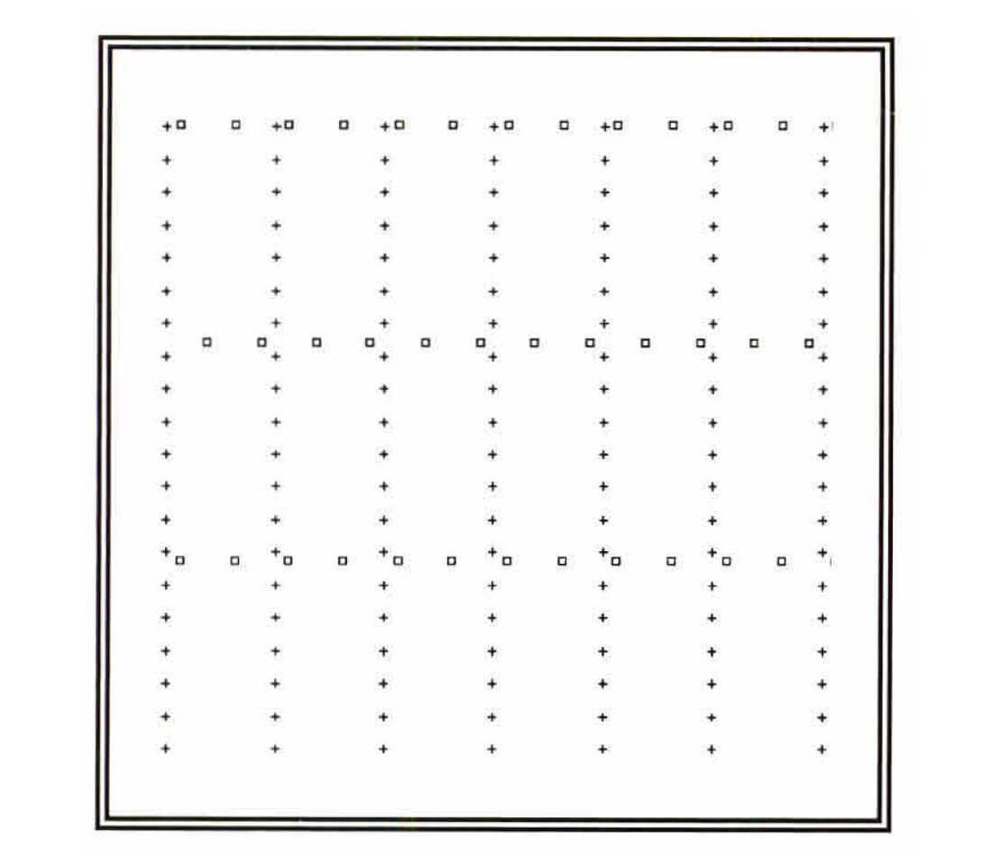
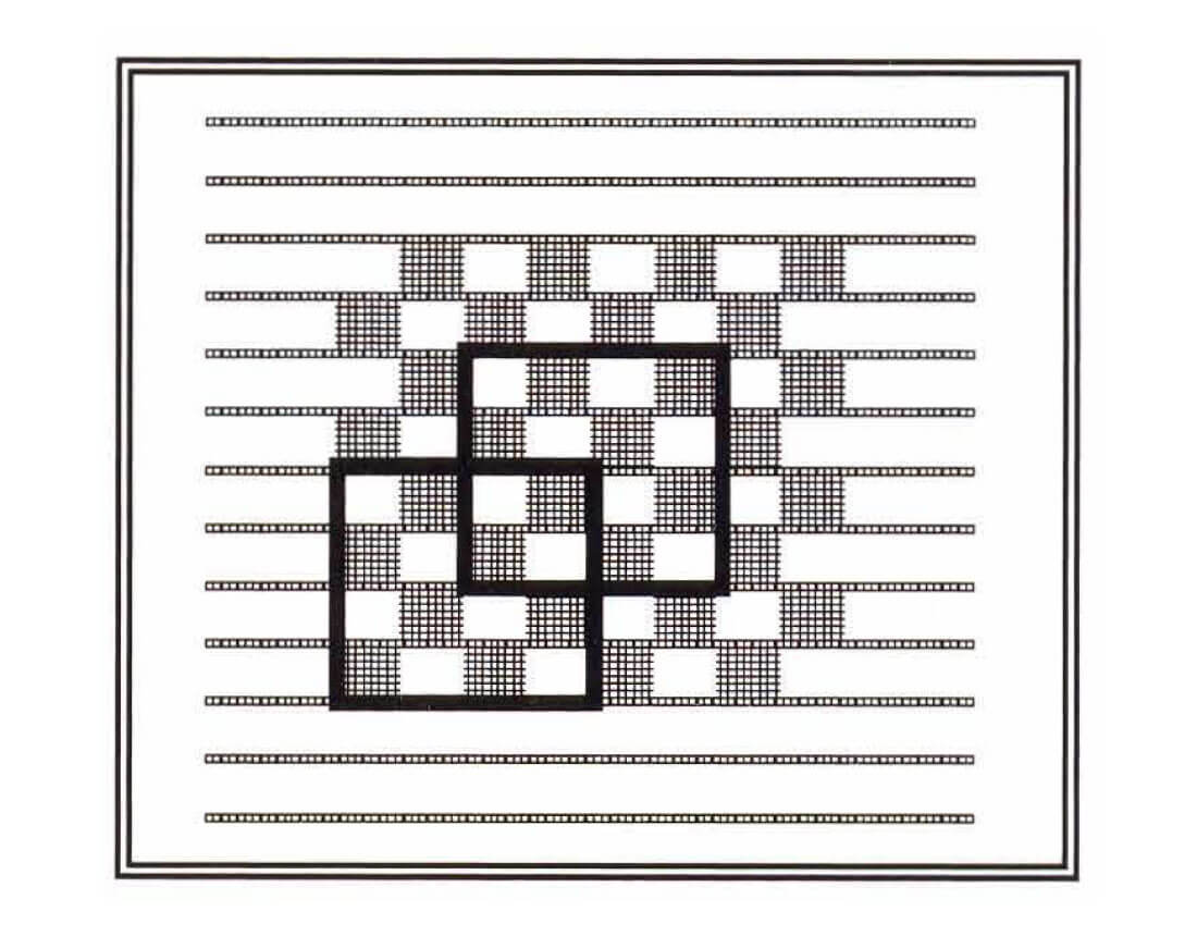
The Bin Fractionation or Flexi-Bin method shown in Figure 6 can be laid out in many different ways (A. Cordsen, 1993). Basically, you must simply ensure that receiver and shot line spacing are non-integral with respect to the group interval. (e.g. Group interval = 60m, SLI=400, RLI=200). Normally midpoints are clustered in the bin centre. In this method an even distribution occurs throughout the bin.
In our example (60,200 ..) you will see 9 groups of midpoints in each CMP bin of 30 x 30. In processing you can choose to stack these "micro-bins" (9 times as many as regular bins), thus achieving much higher resolution (stack trace every 10m, instead of every 30) with consequently lower fold - and therefore potentially lower Signal to Noise ratio.
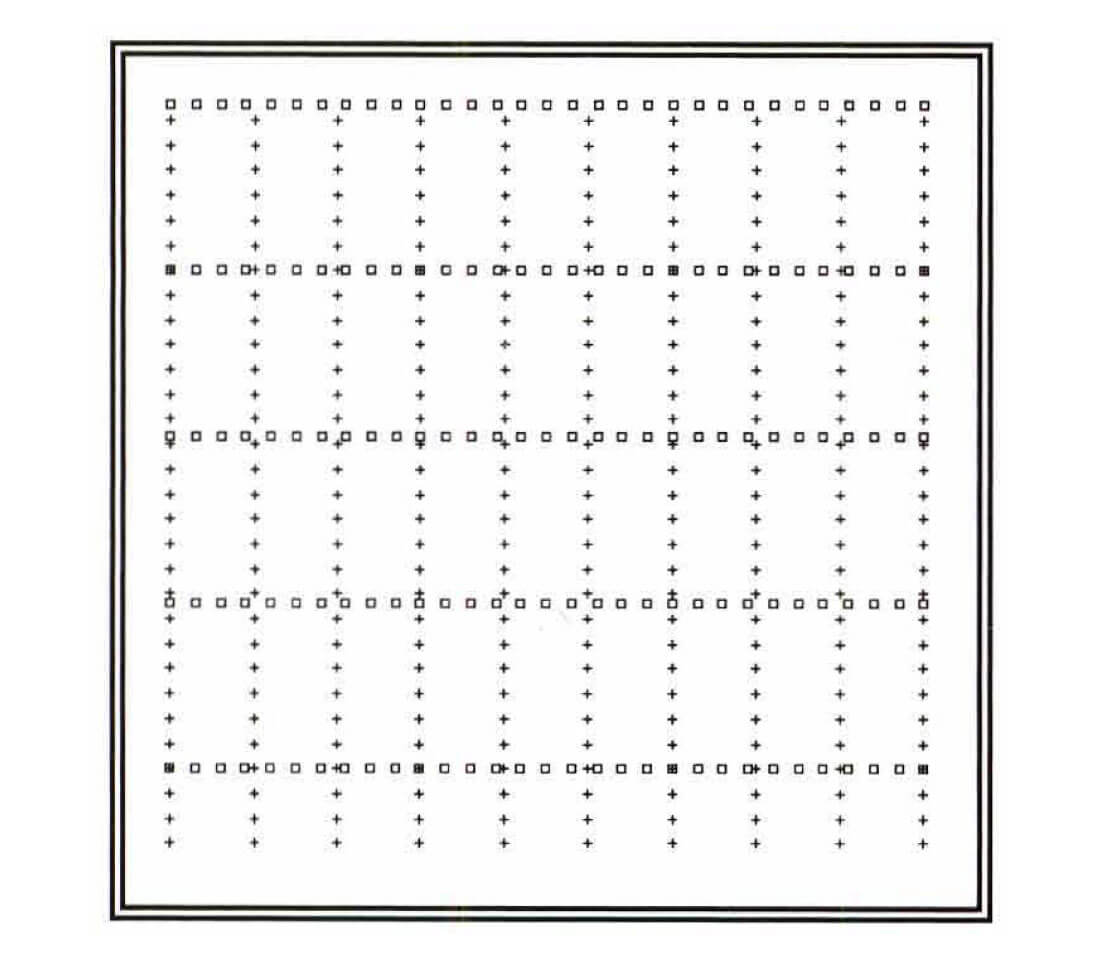
The Button Patch method, shown in Figure 7 was developed by ARCO and is now routinely used in all their 3-D surveys. Each "button" contains a tight pattern of receivers, typically 6 x 6 or 8 x 8. Several buttons are combined in a checker-board pattern to form the receiver patch. Many shots are fired into the receiver patch – often shots all over the survey are fired before moving the receiver patch exactly half its dimension.
Then a lot more shots are fired usually these shots lie between the first group of shots. Operationally not too many receiver moves are required, but of course the shooting trucks (or Vibrators) must travel around the survey every time a new receiver patch is laid out. Laying out extra equipment and shooting twice or even four times on each shot point can alleviate these concerns considerably.
High resolution can be achieved (bunch the receivers tighter). Long offsets, excellent statics coupling, excellent offset and azimuth mix are additional features of this method. Its only real disadvantage is the laying out of the buttons in difficult access areas. The receiver patches are laid out and moved over the area to be imaged at full fold (typically 12 fold is used in these surveys). Shots are placed outside this area to give a taper zone around the edges. Thus at the edges longer offsets are more frequent. After DMO, these move nicely into the edge of the area to be imaged.
Modelling
Using geological modelling we can determine Bin size, Xmin (the largest minimum offset that can be tolerated) and Xmax (largest maximum offset that can be tolerated).
Fold is usually based on the desire for good signal to noise ratio. Signal/Noise for the final survey is: (S/N for one trace) x Sqrt(Fold). So if you double the fold you get a 41 % increase in SIN. Fold should be decided by looking at previous surveys in the area (2-D or 3-D) and remembering that DMO and 3-D Migration can effectively increase the fold as much as 500 times! (Discussed by T. Krey, 1987)
To determine Xmin (the largest minimum offset that can be tolerated) and Xmax (the largest maximum offset that can be tolerated) we can prepare a geological model. Simple ray tracing reveals where reflected energy turns into refracted energy for each event of interest. Thus we can see values of Xmin and Xmax for each event and hence for the whole model.
Other displays help us to determine vertical resolution (quarter wavelength of dominant frequency) and horizontal resolution - Fresnel zone size before migration or the spatial equivalent of the vertical resolution after migration (J. M. Freeland & I.E. Hogg, 1990). We can also see the bin size required to image a desired high frequency on certain dips in the model. Finally recording time and migration aperture (to add to the edge of the survey) should be chosen so that any diffraction patterns from the deepest event of interest will be properly imaged after migration.
Fold vs. Shot Density
Let's derive the basic fold equation for 3-D surveys.
In one square metre: NS shots will cause NS x NC midpoints, where NS = No. of shots/m2 and NC = No. of channels.
If the bin area = b2sq.m.,
FOLD = NS x NC X b2 (midpoints per bin)
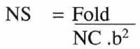
or NS = Fold/(NC X b2)
Example Fold = 24, Bin = 25m., NC = 480, NS = 80 shots/km2
This is the fundamental equation governing all 3-D's. There is an assumption in the derivation that NS shots per sq. meter into NC channels will give rise to NS.NC midpoints inside our square meter. This will only be realised in practise if some of the midpoints arise from shots outside the area being examined and some of the midpoints arise from shots inside and receivers outside the area. This implies that our receiver patterns and shots fired into each pattern must overlap exactly and hence ensure NS.NC midpoints in each unit area of the survey.
If the receiver patterns move (roll-along) in such a way that there is not an exact overlap, you will observe "stripes" of lower fold at regular intervals in your survey.
Receiver Spacing
In the real world we would like all of our receivers to lie within a useable offset range.
Let's assume a centred shot in a patch 2.xr by 2.xr (so the real Xmax = 1.4142 * Xr) If the receivers are spaced 2 b apart, the number of receivers per line = 2 Xr/2 band the number of lines, NL = NCI (2 Xr 12b)
The width of the patch means that 2 Xr and so Receiver line interval, RLI
= NL*RLI
= 2 Xr 1NC/(2 Xr 12b)
= 2 Xr2/NC.b.
Example
Real Xmax = 2300 so Xr = 1600 (approximately)
NC = 480, b = 25 m, RLI = 425 m.
So now we've arrived at an expression linking RLI and NC. We made the assumption that our receivers were laid out in lines RLI apart and that all NC channels had to lie within a useful offset range. The above derivation can easily be modified for narrow swaths where you would include an aspect ratio (inline receiver length vs. cross-line).
Basic 3-D Equations
Combining the above derivations we now state the basic 3-D equations:
NS = No. of shots/sq.m.
NC = No. of recording channels
b = Bin size
Xr = half width (height) of receiver patch
RLI = Receiver line interval
Assumes 100% overlapping patterns in each area of survey - or a regular midpoint density.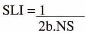
Assumes rectangular receiver pattern - spaced 2b apart. NC receivers in area 4Xr2. Must also have RLI < X min, the largest minimum offset to be found in any bin.
(How else can you lay out NS shots/sq.m.)
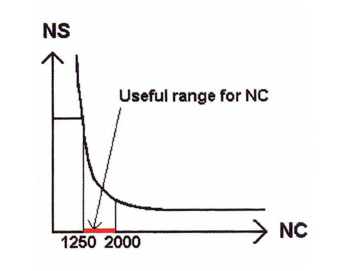
Using the basic 3-D equations we can see graphically how the various parameters are related. Let's assume the following values:
Fold = 25, b = 25 m, Xr = 2500
This leads to:
NS = RLI x 0.08 x 10⁻⁶ (Graph 1)
NS = 0.04/NC (Graph 2)
Let's assume that RLI = 400m. is the largest minimum acceptable offset in any bin. This can be achieved using a Brick or Zig-Zag or any other number of possible strategies.
So to achieve these parameters (Fold=25, b=25m. Xr=2500, RLI=400), we need NS to be in the range of 20 to 32 shots/km2 and NC to be in the range of 1250 to 2000 channels.
Processing Considerations
When you acquire a 3-D survey, the resulting data will require the usual seismic processing flow from statics through stack to migrated stack. How you acquire the data can critically affect your chances of processing it successfully.
Refraction Statics
It is essential that each near surface low velocity refractor be measured by enough source-receiver pairs in all directions. For example, lack of measurements in the cross-line direction (a particular problem in narrow swaths) can lead to "decoupling" of the statics solution from one receiver line to the next. This will appear on the final stack as a geometry "artifact" where data associated with bins along receiver lines are at different times than similar data on adjacent lines.
Reflection statics
Reflection statics require an analysis of the geometry matrix for decoupling as described by Wiggins et al (1976). The concern here is that certain statics wavelengths will be missing from the statics solution because of the particular geometry of the survey. So, a geometry may resolve static changes from one station to the next, but may completely miss, say, the component with wavelength equal to four or eight stations. Again this will show up in the stack as a geometry artifact. An analysis of the geometry to determine that every shot can "see" every other shot through a succession of CMP's and similarly for receivers, will ensure that decoupling will not occur.
Velocity analysis
Use a super bin. All offsets will be grouped by azimuth (for azimuth dependent velocity analysis). So each set of offsets in each azimuth range must define adequate moveout curves ( delta-t > one wavelength) to ensure good velocity discrimination and accurate measurement.
Dip Move-Out
Let h be the shot-receiver offset, V the average velocity and t the time of interest. Then, as shown in Figure 8, the energy at time t in a CMP bin is derived from all shot-receiver pairs which cross the bin and whose midpoints are within h.h/2.V.t of the bin. (Deregowski, Geophysical Prospecting, 1982 pp 318)
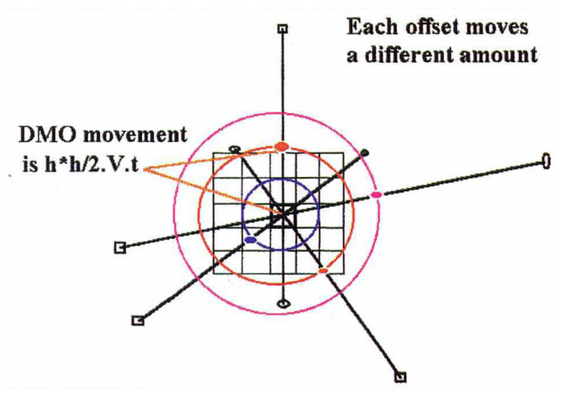
3D DMO needs as many offsets as possible to form the reflections by constructive interferences, otherwise DMO artifacts may occur. These can arise, for example, if a particular set of offsets is missing over a wide area of the survey. In this case, the "smeared" energy from each trace will not combine properly with other "smeared" traces to focus certain dips. In such cases, reflectors with certain dip values may be severely attenuated after DMO.
Fold and the number of unique offsets in each bin after DMO at some specified time "t" is a good measure of the DMO response.
Example:
V=3000 m/s h=IOOO m.
t=1.0 sec.
h2/2Vt = 170m.
or about 7 bins if b=25
Thus DMO has 170m radius at time = 1.0 secs.
Or in other words all traces
- whose offset is 1000m
- whose shot-receiver azimuth passes through a central bin
- whose midpoint is within 170m of that central bin
will each contribute energy to the central bin.
Note that a 5 degree dipping reflector will have its energy shifted a horizontal distance of (h2/V.t).sin θ.cosθ - or using the above V, t and h we get 15m.
Multiple attenuation
A good mix of offsets from near to far will attenuate multiples through CDP stacking.
Stack (noise rejection)
A good mix of offsets will attenuate noise which is not consistent from trace to trace.
Field Layouts - Pros and Cons of the various layout strategies.
| Layout | Pros | Cons |
|---|---|---|
| Straight | Simple Geometry. | Near trace gets large in centre of "box" |
| Swath | Simple Geometry. Cost efficient. Minimum equipment movement. | Poor offset + azimuth distribution. Poor statics coupling. |
| Brick | Better near trace -> wider RLI. Reasonable offset and azimuths. | Access can be a problem. |
| Zig Zag | Same as Brick. Efficient for equipment moves. | Must have very open access. |
| Bin Fract. | High resolution with low fold. Super Bins for normal use have good offset and azimuth mix. | Same as Straight. |
| Button | Efficient utilization of large channel systems. Achieves tight spacing with excellent offsets and azimuths. Good statics coupling. | Can require large number of shots over a wide area for each patch. |
| Odds/Evens | Special case of Brick without such severe access problems. Better offset and azimuth. | Twice the shot lines as conventional straight shoot. Only half the shots are taken on each line. |
| Radial | Good for salt domes. | An operational and processing nightmare. |
| Hexagon | Layout hexagonal receiver patches and use hexagonal CMP bins. More efficient use of equipment since more channels will be at useful offsets. | The juggie can't spell hexagon. |
Practical Considerations
Modem field systems such as the I/O System One and Two can be controlled by so called script files. Obviously the computer program used for designing the 3-D can generate such files which specify the receiver stations to be turned on with certain shots.
When a seismic crew starts up they will layout cable until there is enough to start taking the first shot. Thereafter receiver cable is moved at the same time as shooting occurs. This first (and last) shot situation can be quite a time waster, especially for large multi-channel systems. A crew can save time and money if they start shooting earlier - as is the case when you do a roll on/off.
The direction in which receiver cables are laid out can dramatically affect the logistics of a survey. For example with a long skinny survey, it can be advantageous to layout receivers across the shorter dimension. Then take all the shots for the patches at one end, roll up one line and take the next shots all the way across the survey - and so on. This advantage usually occurs when the receiver patch is the entire width of the survey.
Field Example
Before the example 3-D was shot, the designer made a careful analysis of the CMP fold for different offset ranges. This revealed some severe inadequacies in the fold of the near traces (0 - 800m). The fold for offset range 800 - 1600m showed no real problems, as did the fold for 1600 - 2400m. Extra shots were added in various places to cure these problems - and to compensate for real life problems - namely a small lake in the South East comer and a river which cut right through the centre of the survey. Digitiser input from maps eased this task. Shots were moved, added etc. and the resulting fold maps for the various offset ranges recalculated.
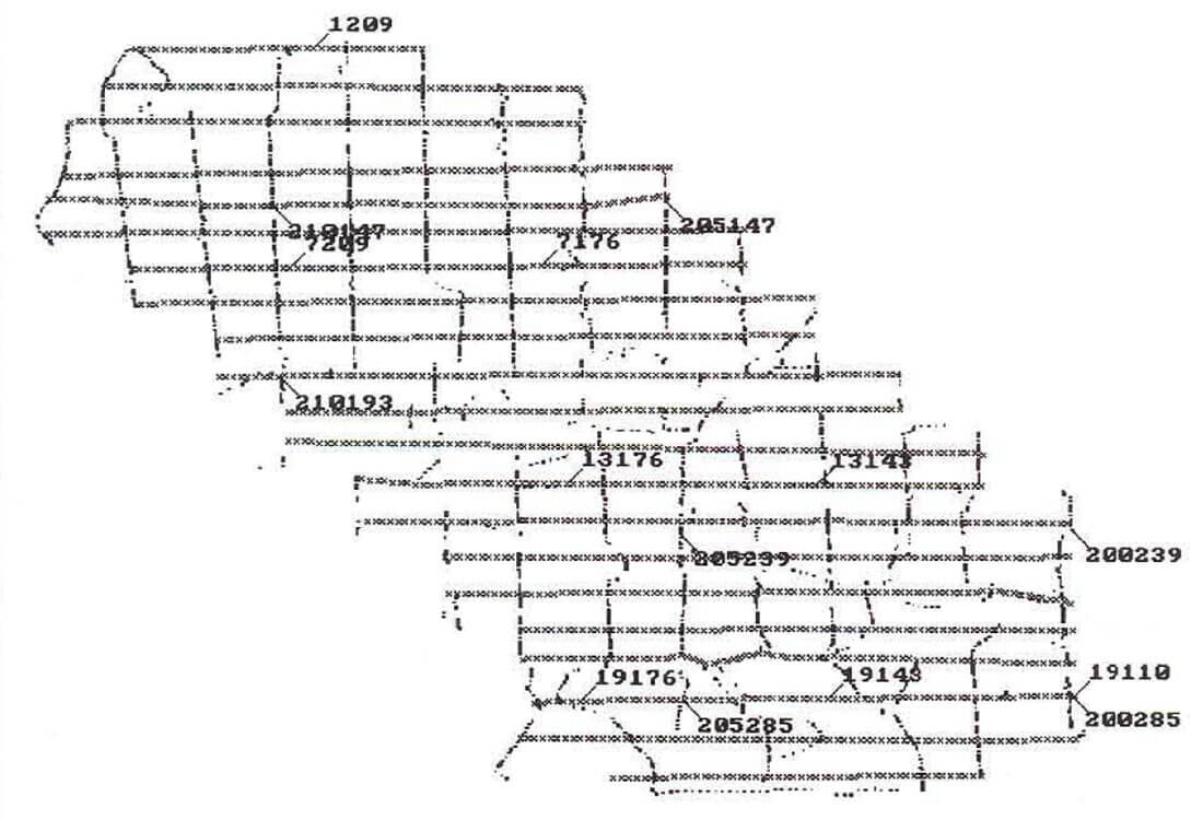
After the survey was shot, the survey information in the form of a SEGPI file was input to the computer program. This is shown in Figure 9. We then calculated the CMP fold for all offsets in the range 0 - 2400m. Very few problems remained on this final version and we congratulate the survey designer on a job well done.
Common Depth Points
In the real world the energy from a reflector does not necessarily come from that piece of the reflector which is halfway between shot and receiver (CMP). DMO corrects traces from their CMP (Common Mid Point) position to the CDP position and it is certainly of interest to know how well we are illuminating each piece of the target. This is the so-called CDP Fold. 3-D ray tracing is essential for true CDP analysis.
Future Directions
3D's are expensive and a lot of current research into layout methods is focussing attention 011 ways in which we can cut costs and still achieve our geophysical objectives. Any 3D geometry must be seen as a measuring instrument which has a "resolving power" for such things as statics solutions, velocity discrimination, dip resolution and so forth. Lay out methods are currently largely tied to existing technology with cables, central recorders etc. Future technology such as telemetry, GPS location of shots and receivers will open up new possibilities. The most intriguing of these involve methods where we place shots and receivers (carefully) at random!
Conclusions
- Use geologic modelling for Xmin, Xmax, Bin size, Migration apertures, and Recording time.
- Ensure regular shot density (Shots per square Km.).
- Ensure 100% overlapping receiver patches (this will ensure even midpoint density - hence even fold coverage).
- Keep all offsets in the range (Xmin, Xmax). 5. Shots and receivers should be "tied" through CMP's to ensure statics coupling.
- Unique offset fold should be close to actual CMP fold - essential for DMO.
- Offset mix in each bin must be adequate for NMO (velocity analysis), DMO and stack (noise rejection).
- Calculate cost for each strategy. 3D's in the desert won't work,in the jungle!


Join the Conversation
Interested in starting, or contributing to a conversation about an article or issue of the RECORDER? Join our CSEG LinkedIn Group.
Share This Article