3D Model Evaluation by Data Simulation

In the past, we have separated 3D programs into discrete stages. In the design and modeling phase, we look at plots of fold, offset and azimuth statistics to speculate whether a model is of sufficient quality to map an objective. The acquisition phase often seems to be devoted to perturbing the model up to or beyond its limits. The processing phase is the black box and the processors are the brave souls who everybody expects to “fix” their data. The interpretation phase is where we find out to what degree we overspent (too dense a model, data is excellent, could we have spent less money and obtained the same results?) or underspent (tried to save too much money with a sparse model and now we have to blame somebody).

When 3D models fail (which is mercifully rare), they either fail catastrophically or statistically. A catastrophic failure is one where data is virtually useless; we abandon the seismic as a guide in our exploration effort and pick well locations based on alternate data sources. Fortunately, I have only been party to two such surveys in my career. This is often better than the alternative type of failure in that we only lose the money invested in the seismic.

In a statistical failure, we generate geometric imprinting ... or perhaps we leave unresolved multiples in portions of our prospect ... or perhaps AVO effects are missed or misinterpreted due to perturbations in statistical sampling. These are dangerous failures in that they are not obvious to the interpreter. The data seem to be good, but the interpreter is misled by artifacts. Too often, we end up drilling expensive wells as a result of these artifacts. The results are confusing, difficult to reconcile in postmortems, and we lose confidence in the seismic (as well as losing a large amount of exploration capital in an abandoned well).

Conventional 3D modeling produces plots such as fold, offset distribution and azimuth distribution. The designer must make qualitative judgments on the significance of the plot. “Does the numerical fold accurately represent the processed fold at the zone of interest?” “Is a model with uniform offset distribution better than one that produces clumpy distributions?” “If so, how much better?”

However, the real impact of these statistics on the interpreted data depends on their interplay with the characteristics of the actual data. To what extent are multiples required to stack out? Does our major noise come from slow ground roll in the near offsets or apparently fast guided waves at the far offsets? What is our amplitude decay with offset for our target in this area? What is the actual useable offset range at the zone of interest after muting and NMO correction?

In figure 1, we have created a model with variable grid spacing. Fold has been calculated and is displayed as a color ranging from red (high fold) to blue (low fold).

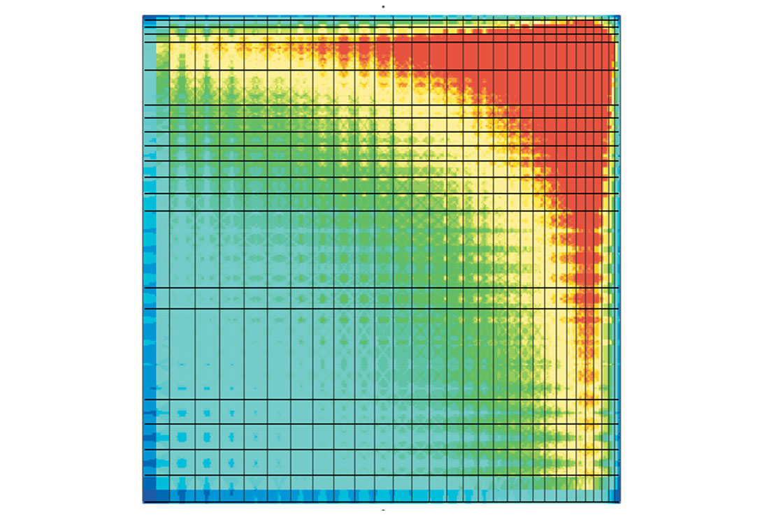
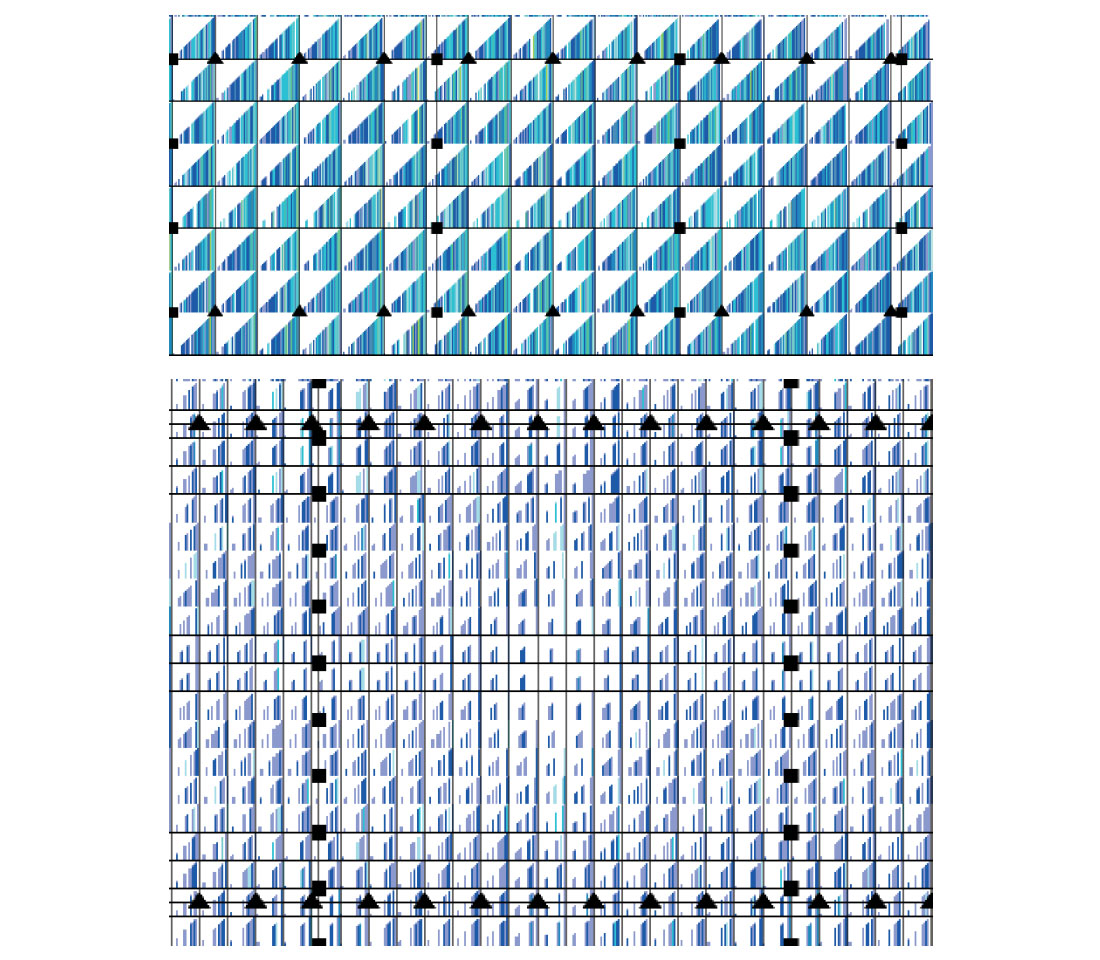
So now we can see the variability of fold, but how do we know what is acceptable or not for our target horizon? We can examine more statistics ... figure 2 shows offset distribution plots for the two opposite corners of the model. The high fold corner (top of figure) shows regular offset distribution with all offsets evenly sampled in each bin. The low fold corner (bottom of figure) shows erratic offset distribution with a high degree of heterogeneity from bin to bin.

Although they analyze the model quantitatively, these model-based statistics still do not clearly indicate at what point we can expect our data to deteriorate. That will depend on the data in this prospect area, with its own characteristic signal to noise ratios and offset dependent signal and noise character. It will also depend on the nature of the target we wish to examine.

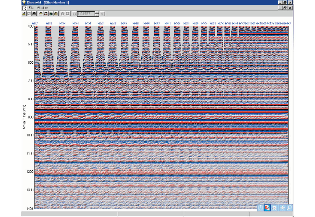
By obtaining a sample of existing data from our prospect area, we can simulate a stacked data volume using the sample data and the offset statistics from the proposed model. Pre-existing 2- D data passing through the proposed 3-D area is usually available and is often recently re-processed. Typically, we generate a low-fold common offset stack after all normal moveout and statics corrections have been applied (selected from an area believed to be representative of the data quality for the prospect). The model based offset distribution for each bin is used to determine which traces from the reference data should contribute to each simulated stacked trace. In this manner, any arbitrary line can be simulated.

Geometric imprinting manifests itself in a variety of characters in this model. Note that the strong reflection near 925 ms is quite stable throughout the model. Obviously, the shallow reflections above 650 ms suffer greatly in the sparser grids due to lack of near offset sampling. The package of reflectors just above 800 ms exhibits amplitude imprinting for most of the model except at the finest sampling (rightmost third). The reflector at 1050 ms suffers from incomplete multiple suppression for the sparser grids. The optimum grid depends on the interpreter’s zone of interest and imaging requirements.

At the design stage, we now endeavor to show the interpreter what his final data may look like in the presence of geometric artifacts (everything except the geology). This analysis is a great asset in better defining the optimum 3D model on a prospect-by-prospect basis. It is a valuable tool for evaluating the impact of perturbations to a planned survey (permit lockouts, etc.).

We also recommend that this simulation be conducted for completed surveys using the “as built” survey files. The interpreter should use the simulated data as a reference when he is studying the final processed data set. The simulated data will help identify areas of potentially misleading character due to geometric distortions in the acquired data.

We believe that stacked data simulation allows us to more precisely define that delicate balance between optimized survey cost and image quality. We also hope this method may help quantify the risk associated with interpretation of marginal 3-D designs.