A New Approach to Pore Pressure Predictions Generation, Expulsion and Retention Trio: Case Histories

A comprehensive framework and fresh perspective to pore pressure prediction methods and algorithms based on the established geological building blocks is presented. Applying the suggested four subsurface zones is the backbone of this pore pressure prediction approach. Determining the boundary of the four subsurface zones utilizing seismic data is crucial for selecting the appropriate method and algorithms for pressure prediction.

This approach divides the previously so-called normally pressured upper section into two zones: namely hydrostatic and hydrodynamic. Consequently, data in the hydrodynamic section is used to establish the compaction trend and not the entire section above the top of geopressure. The section below the top of geopressure is divided into transition and geopressured zones. This method calculates the compaction trend, rather than graphically displaying it for calibration purposes. Moreover, it eliminates the confusion of extrapolating the predicted effective stress values above the top of geopressure.

In this paper, entrapment represents the main cause of overpresssure buildup. Fluid pressure inflation due to stress, aqua-thermal and dewatering processes is the genesis and not the outcome. The effective seal is the main mechanism for creating excess pressure. Investigating possible breach of the seal due to subsurface structural failure is a key objective for pore pressure prediction.

The subsurface hydro-geological zoning greatly impacts the velocity, resistivity and density profiles. Seismic velocity to pore pressure transformation modeling foresees the trio process from generation to expulsion to entrapment before drilling the prospect. The newly introduced subsurface partitions, trio concept, algorithms, and predictive modeling incorporated with the geological setting are supported by case histories from the Gulf of Mexico.

Introduction

Pore pressure prediction is the ability to create numerical formulas that mimic the subsurface pressure profile. However, without establishing the geological groundwork for these mathematical equations, results can be misleading. The subsurface pore pressure build-up partitions are mainly caused by stress and compartmentalized lithology in an aqueous environment. Stress and fluid expansion (due to aqua-thermal and diagenesis) alone cannot be the only trigger mechanism for pore pressure ramps build up (shift from normal to abnormal pressures). These ramps create a pressure surge with hard kicks that sometimes exceeds 3000 psi (20.691 MPa). Leftwich and Engelder (1994) show several examples of these pressure ramps in the Gulf of Mexico Coast area. The thorough examination and analysis of the GOM data from wells with competent seals, as well as breached reservoirs, all point to an overpressure mechanism composed of three phases. The trilogy processes of genesis, exodus, and retention have to be fulfilled for the occurrence of excess pressure (overpressure) in the sub-surface to take place.

The vertical generic pore pressure profile in the subsurface (Figure 1) can be, in most cases, divided into four zones (Shaker, 2012) namely: free flow, hydrodynamic, transition and geopressured (A, B, C and D respectively). This is contrary to the inherited conventional assumption established by Fertl (1976) of two subsurface zones, namely: hydrostatic and abnormally pressured.

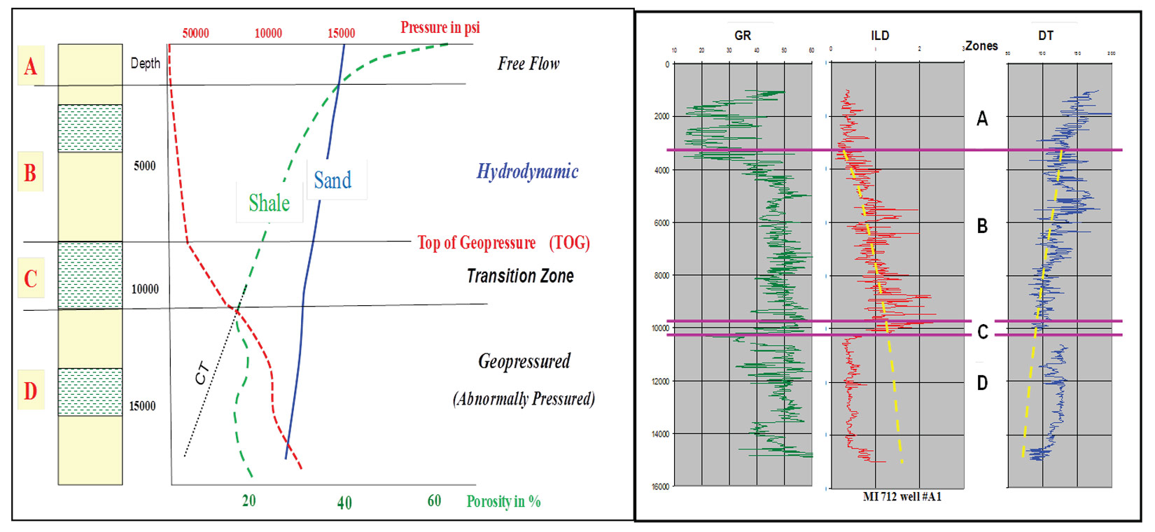
Fertl (1976), Magara (1976), Swarbrick et al (2002), and Tingay et al. (2009) discussed numerous causes of pore pressure generation, all of which lead to an increase of in situ fluid pressure. Trapping causes the excess subsurface geopressure, prior to the complete expulsion process taking place. The lack of seal (zone C) leads to breaching and venting of the over-pressured fluids (water and hydrocarbon) to the sea floor or ground surface without regard to the mechanism of pressure source.

Most of zone C sediment, which is the main cause of excess pressure, is deposited as fine sediments (e.g. shale) and is usually associated with a high stand environment. Sturrock (1996) indicated that the deposition of widespread pelagic shale is related to high sea level. It usually coincides with maximum flooding surface (deep seated) shale deposits, e.g. the Cibicides opima shale offshore Texas (Shaker, 2008), and the Bigenerina A. in the lower slope shale formations offshore Louisiana (Harkins and Baugher, 1969). This is contrary to the idea of a high depositional rate sequence, which is mainly built of coarse sediments, as the cause of geopressure. Swarbrick et al. (2002) stated that “the FRD (Fluid Retention Depth) is shallow where the sedimentation rate is high, leading to high magnitude overpressure (low effective stress) at depth.” Sediment load might accelerate the rate of vertical stress and temperature, but does not cause the excess pressure entrapment. Dutta (1987) stated “if there is one word that can describe the chief geological aspects of geopressure, it would be ‘stratigraphic’.”

Below the transition zone C, the geopressured system (zone D) is usually compartmentalized by seals older than the top seal and the reservoir quality beds that bear the excess hydrostatic gradient (fluid at rest) in a cascade fashion (Shaker, 2012). In this zone, formation fluids are entrapped under the seal and bear an excess static pressure. Fluid is trapped below the pressure cap and does not flow in the same reservoir but carries a portion of the overburden (i.e. effective) stress.

Most of the conventional prediction methods (e.g. Eaton, 1975; Bowers, 1994) use the section in zones A and B (the so-called normal compaction trend, NCT) as the lead track for their calculations in the geopressured zone D. A unique mathematical calculation is introduced here to establish the compaction trend (CT) instead of the manual graphical extrapolation. Eaton (1975) stated in his conclusion that “the methods used to establish normal trends vary as much as the number of people who do it”. Unfortunately, after forty years, geopressure analysts still sway, break and use average values to establish the NCT.

Geology – Hydrology – Geopressure: The Impact of Geological Process on Hydrology and Pore Pressure

Fluvial, deltaic, terrigenous shelf slopes, and deep water basins are widely explored for oil and gas in which geopressure analysis is one of the useful exploration tools. A generic subsurface hydrogeological – geopressure profile partition follows:

Zone A: Rubey and Hubbert (1959) stated that, for depths of 1 to 2 km, pressure is a function of depth where fluid moves freely and exhibits a hydrostatic pressure gradient derived from the weight of the water column only. The pressure gradient in Zone A in the Gulf of Mexico is 0.465 psi/ft (10.52 MPa/km). Velocity stays in the range of 5000-5500 ft/sec.

Zone B: This zone starts at a depth where the overburden’s stress promotes the fine sediments to start the process of dewatering. Depth, rate of sedimentation, porosity, water and frame pressures are the main factors of the water flow rate decreasing with depth and time. The GOM pressure gradient in zone B ranges from 0.52 psi/ft to 0.59 psi/ft. The lack of complete grain to grain contact combined with fluid movement can be simulated by the stage B model of Terzaghi– Peck (1948) where 0.465 < λ < 1 (λ is the ratio of pore stress to total overburden stress). Velocity starts the exponential increase at the top of this zone, and shows the reverse trend at the base.

Zones C and D: Below the top seal, multiple methods have been established to calculate the geopressure (e.g., abnormal, overpressure, excess pressure, hard pressure, etc.) from cross-plots (Hottmann and Johnson, 1965; Mathew and Kelly, 1967), tracing overlay (Pennebaker, 1968), algorithm-based methods (Eaton, 1975; Bowers, 1994), and rock physics modeling (Dutta and Khazanehdari, 2006). The widely used conventional effective stress prediction methods are usually categorized into two groups, ‘horizontal’ and ‘vertical’. They mostly rely on the departure of the measured velocity, resistivity, and density values (V_o, R_o, and ρ_o) from the equivalent extrapolated normal values (V_n, R_n, and ρ_n). The horizontal effective stress of Eaton (1975) is used in this study to estimate the pressure in zone C and D. The preference of using Eaton’s method instead of Bowers’ is due to the fact that vertical methods, such as Bowers’, assume that the effective stress is equal above and below the top of geopressure. Moreover, Bowers’ method needs three calibration parameters (Vo, A, and B) with the “local data.” Bell (2002) stated that “application of equivalent-depth methods predicts too large an effective pressure and thereby underestimates the pore pressure.”

Pore Pressure Calculations: Predictive Modeling Before Drilling

Defining the four zones before drilling

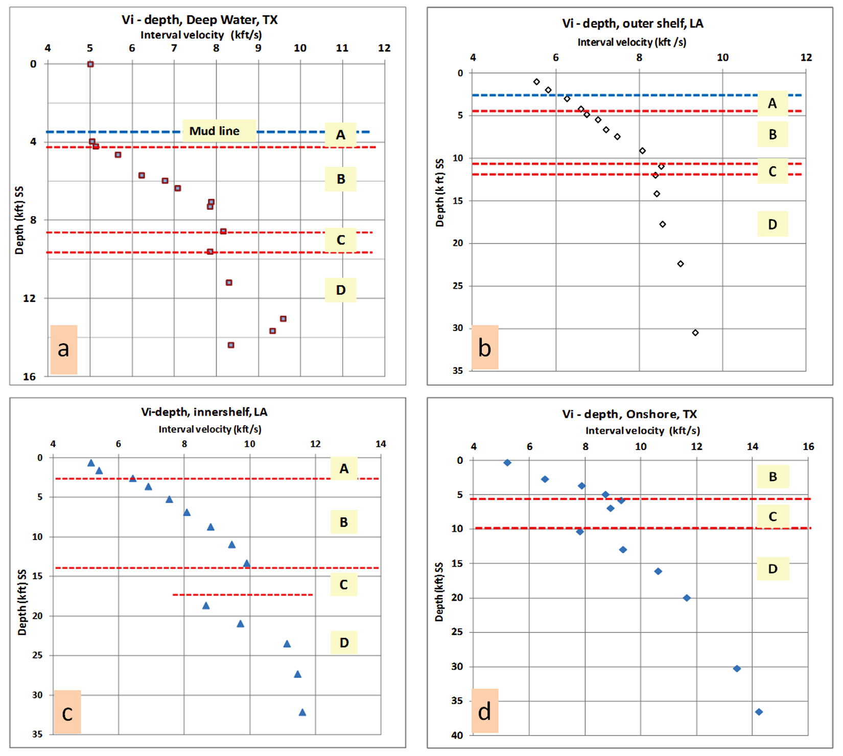
Compressional seismic velocity (V_p) is the first petrophysical property that can be used to predict the depth to the previously-mentioned four zones. The normal moveout and RMS velocities can be used for a quick look and regional assessment. However, interval or Dix velocity (V_i) is the velocity recommended for 1D and 2D interpretations. Quality control displays such as NMO-corrected gathers should be used to check the accuracy of velocity picks but never to make predictions based on single velocity function (Dutta, 1999; personal notes). Velocities must be processed for de-multiple, DMO (dip move-out) and pre-stack migration. Converting the time-velocity pairs to depthvelocity pairs is the first objective and need to be calibrated against check-shot, velocity survey and/or sonic logs from offset wells. Outlier velocity values representing calcareous beds, salt inter-beds, gravel, thick sands and pay zones should be eliminated from the analysis. Figure 2 shows velocity pairs from different depositional environments, ranging from deep water, outer and inner shelf, to onshore, and the estimated depth for each of the four zones.

Calculating pressure in zones A and B

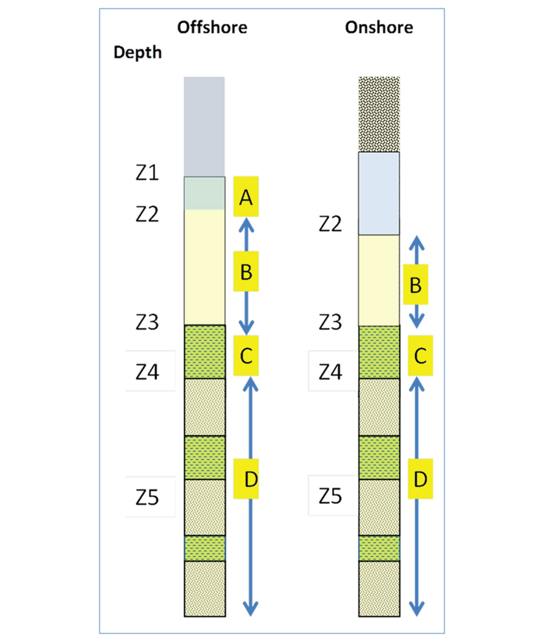
Deep water: it is assumed that there is an offshore wildcat trajectory and pressure will be calculated at specific depths in each zone (Figure 3). In case of onshore wells, calculation starts from the water table in the already compacted zone B.

Calculating pressure in zone A: the top of zone A is at the mud-line (z₁) and the base (z₂) is where the velocity values begin the gradual compaction trend.

Pressure at the mud line (Pz₁):

where ρ = density of seawater, g = acceleration due to gravity, z₁ = water depth, and 0.4335 is the pressure gradient conversion from g/cc to psi/ft.

Pressure (psi) at the base of zone A (Pz2):

where ρ = density of shallow formation’s water ≈ sea water.

Log measurements are frequently unavailable due to driving the surface casing string (36 inch) into zone A.

Pressure estimate in zone B: all the previous methods calculate the pressure in zone B as if a normal hydrostatic pressure exists. In this paper, a new estimation method is introduced to calculate pressure in this hydrodynamiczone. The hydrodynamic pressure value at certain depth is a function of permeability and differential pressure between the bottom and top of each compartment in this zone. The pressure estimation in B zone follows Darcy’s Law. The discharge segment B begins when and where the fluid pressure exceeds the hydrostatic gradient due to the increase of sediment load, grain to grain contact, and in situ pressure. The effective stress theorem is applicable only if fluid is at rest (hydrostatic gradient) and is not flowing (e.g. stage A in Terzaghi and Peck, 1948 model where λ = 1). Empirical correlation between velocity trends in the so called normal pressure section (A and B zones) and ΔP was not important according to previous studies. This is a result of the assumption that the entire section above the top of geopressure (TOG) is hydrostatic and normally pressured.

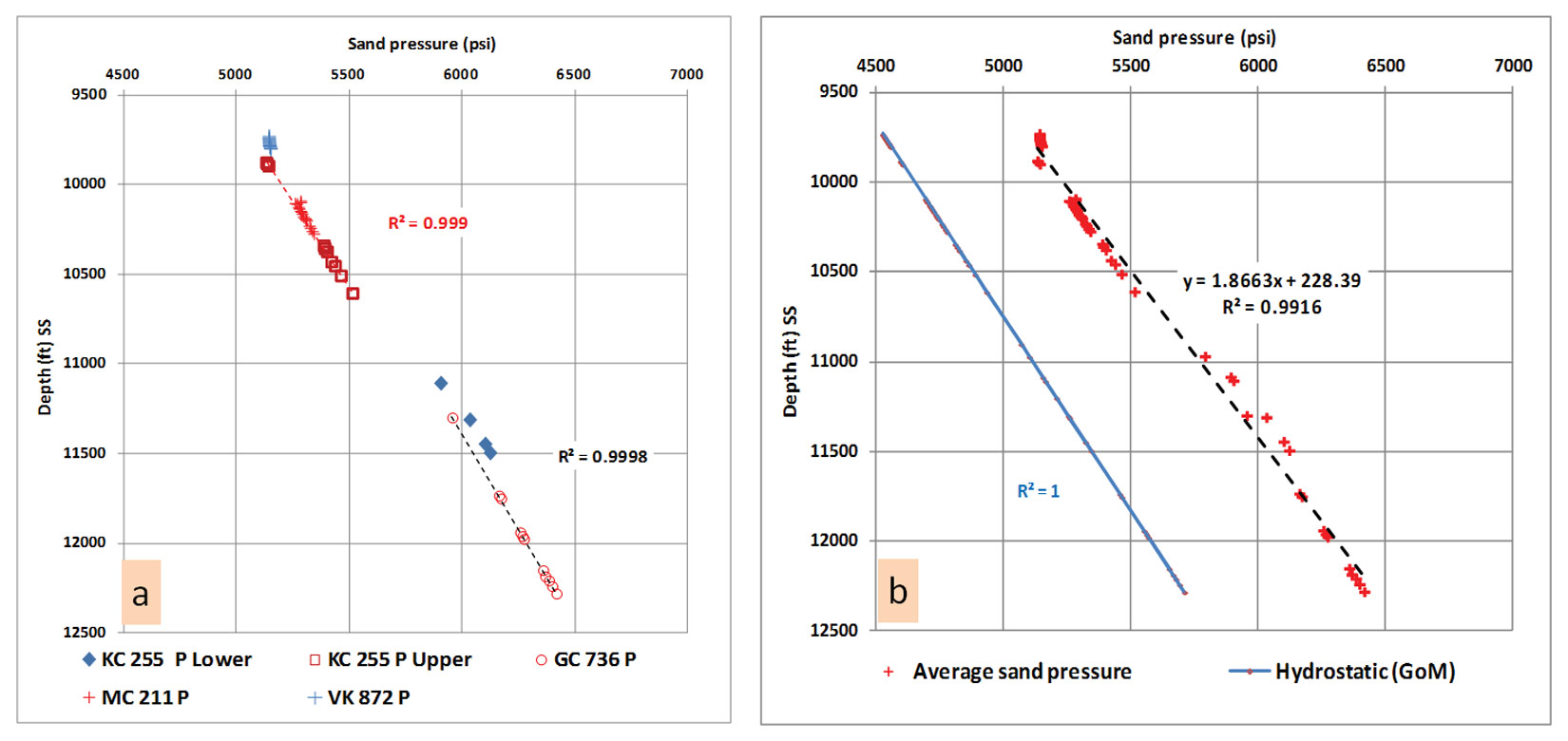
Calculating the pressure in this zone is an intricate mission, especially in a wildcat area, since it requires offset data for calibration. The depth to top of zone B starts where the velocity exponentially increases in response to the decrease of porosity with depth following Athy’s (1930) relationship. The top of zone C starts where the velocity trend reverses its course (Figure 2). Establishing the mathematical relationship between the extent and slope of zone B from seismic velocity and pore-pressure values is a key solution. Occasionally, repeated formation tester (RFT) and modular formation dynamic tester (MDT) measurements were taken from this zone’s sand beds in different deep water wells in the Gulf of Mexico. They show a clear upward hydrodynamic flow (Figure 4) with a higher gradient than the GOM hydrostatic gradient and the hydraulic head reaches above the mud line (Shaker, 2012).

Mud weight (Figure 5) increases from 8.9 ppg at the base of zone A to a value sometimes exceeding 11 ppg at the intermediate 9 5/8 inch casing seat (TOG) to encounter the up flow. It is observed that the pressure gradient in zone B is higher on-shore (older sediment with less flow) than offshore, especially in deep water.

Measured pressured data collected from Mississippi Canyon (MC), Green Canyon (GC), Keathley Canyon (KC), and Visco Knoll (VK) are used. The gradient in the Pleistocene deeper section in KC and GC areas shows higher values than the shallow Pleistocene section in the KC, GC, and VK areas. The overall data values for the above mentioned areas (Figure 4b) show an average gradient of 0.536 psi/ ft and hydraulic head of 230 ft if sand flows freely to the sea floor (mud pressure absent). Predicting the sands’ pressure in this zone is important to avoid any unexpected water flow during drilling. From Figure 4a, sand pressure in the shallow Upper Pleistocene at depth z3 can be calculated as:

and sand pressure in the deep Upper Pleistocene at depth z₃ can be calculated as:

From Figure 4b, the average Upper Pleistocene sand pressure (psi) at any depth (z₃) within the B zone can be calculated as:

Mud pressure gradually increases to compensate for the pressure difference between the high flow sand and the low permeability negligible flowing shale. Pressure in sand follows a linear upward flow (equations 3, 4 and 5) and the shale pressure follows an exponential trend (Figure 1) reflecting the reduction of porosity (Athy, 1930). Usually, mud weight is raised at the shale-sand interface where drilling events requires mudding up.

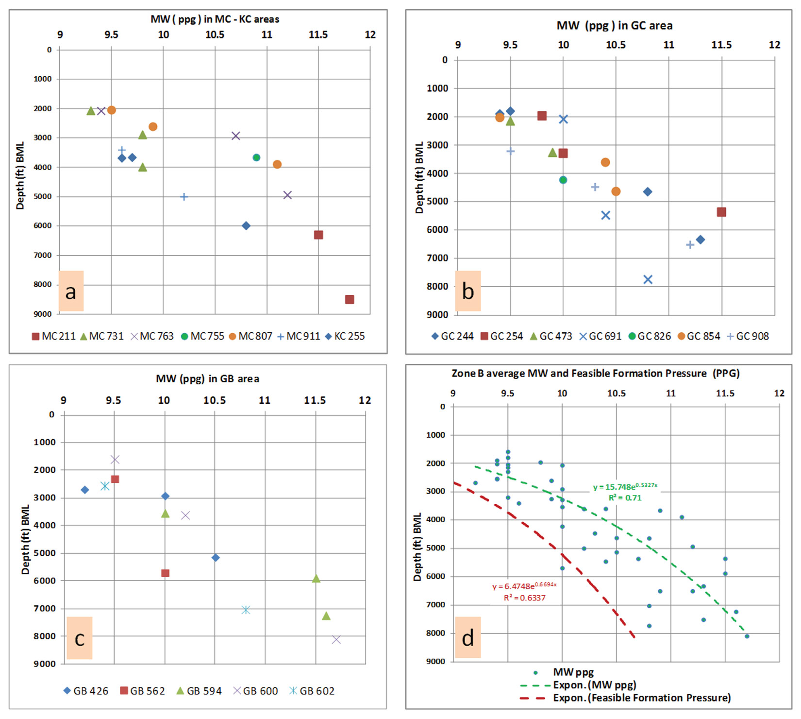
The average formation pressure of sand and shale (feasible formation pressure) in this zone is estimated from the populated MW data sets. The mud pressure (ppg) at any depth (z₃) within zone B, is calculated from mud weight values of MC, KC, GC and GB areas (Figures 5a, b, and c). On these plots, the depth value data (y axis) are in reference to the mud line due to the wide range of subsea depths to mud lines. The average mud pressure (Figure 5d) required for keeping the borehole stable and avoiding any formation water flow follows an exponential trend as the least squares best fit for the data ranges from 9.15 to 11.7 ppg, and can be calculated as:

Pz₃ mud pressure (ppg) at any point within zone B (BML)

where constant α for this data set is 5.18 (R² = 0.71).

Equation 6 was calibrated and validated using known mud weights from numerous offset wells.

The estimated average feasible formation pressure (FFP) was gauged by mud weight pressure from wells drilled with balanced mud when Shallow Water Flow was not reported. It is based on the drilling practices and safety regulations that are constrained by formation and fracture pressures. Mud weight is usually 0.5 ppg greater than the before drilling predicted pore pressure at the second casing string (20 inches) and 0.75-1.0 ppg greater than the predicted pressure at 16 to 13 3/8 inch casing strings and the intermediate casing. The FFP therefore follows the same exponential trend (Figure 5d). The average FFP (ppg mwe) at any depth below the mud line (z₃- depth BML) in zone B is calculated as follows:

where constant α is 2.79 (R²= 0.63).

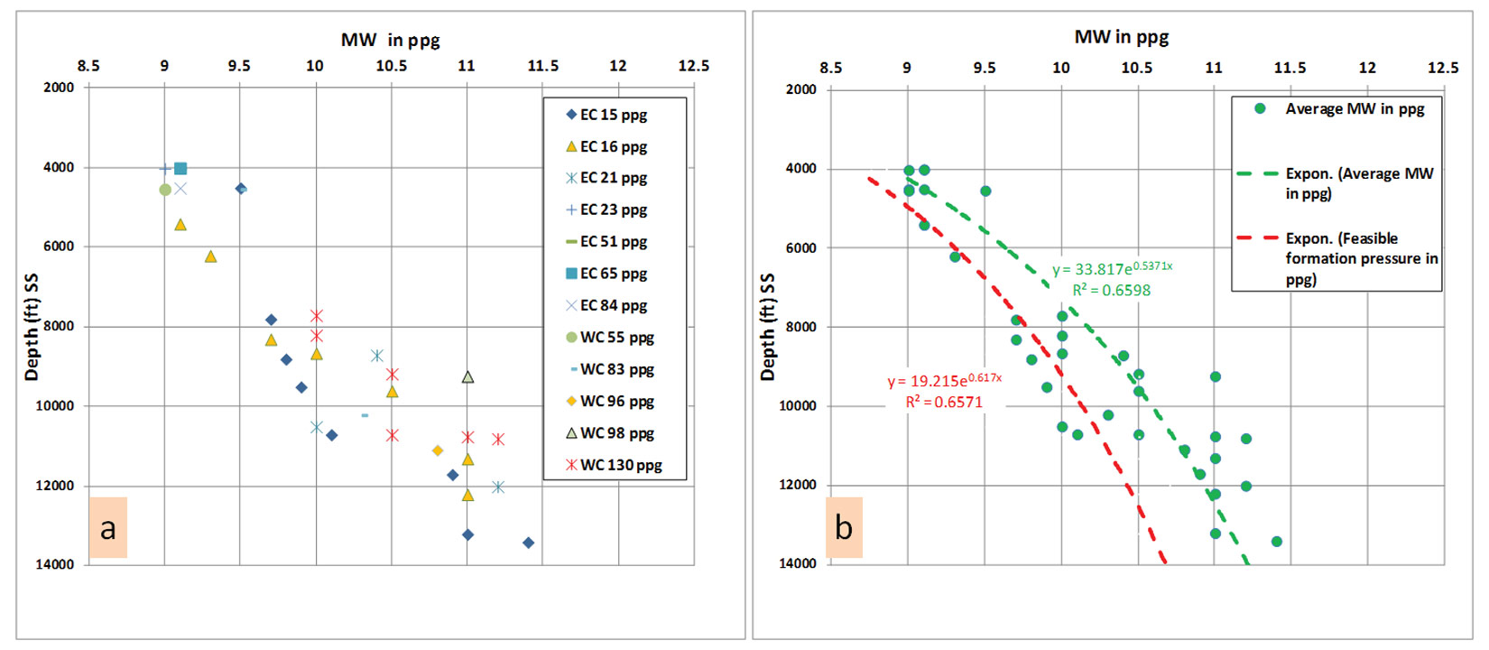
Offshore shelf: on the shelf, the mud weight required to penetrate this zone ranges from 9.5 to 11.5 ppg (0.492 to 0.6 psi/ft). This mud data was collected from several wells (zone B minimum depth is ~4000 ft) in East and West Cameron, offshore Louisiana, and Gulf of Mexico (Figure 6). The least squares fit through the data set from twelve wells in this area (for pressures ranging from 9 to 11.4 ppg and depths ranging from 4000 to 13500 ft) is exponential.

The constant, α, for this E-W Cameron data set is 6.63 (R² =0.66).

The feasible formation pressure (FSS) is calculated as drilling and regulation practice requires.

FFP is deduced from mud pressure within zone B, in ppg,

The constant, α, for this E-W Cameron data set is 4.8 (R2 =0.66).

The MW and FFS trends on the shelf show more proximity than the deep water trends since the hydrodynamic flow has reached relative stability due to the older age of the sediments, and due to the shallow water depth (40 to 60 ft).

Calculating pressure in zones C and D

The effective stress theorem is applied to the data below the top seal because the fluid is trapped in the subsurface in different compartments. A new method of calculating the modified compaction trend (CT) integrating with Eaton’s algorithm is used in this study to predict pressure in the C and D zone. The velocity is calculated as if the compaction trend is extrapolated to the targeted objective to attain the Δt_c values. Figure 7a exhibits the entire seismic interval velocity set (converted to sonic slowness as Δt_o) and the extrapolated compaction trend values, as Δt_c, for a super-gather’s velocity in close proximity to a well drilled in the offshore TX inner shelf.

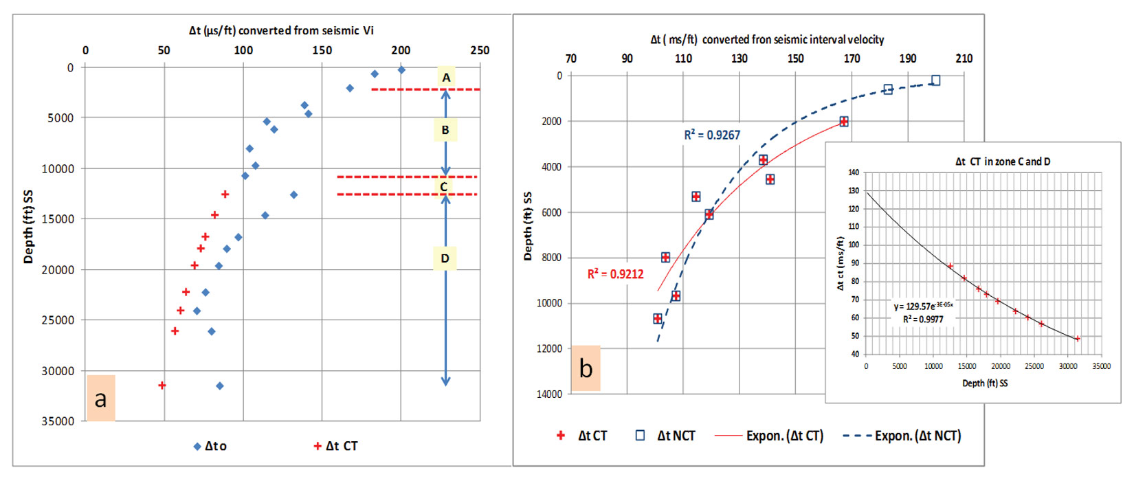
The average Δt_c was calculated and extrapolated to zone C and D from the exponential trend (Figure 7b) as:

This is a unique equation and only applied to this depth-V_i pair at this CDP only.

Eaton’s equation (1975) is applied in zones C and D as follows:

where P/z₄ is the predicted pressure gradient, S/z₄ is the overburden gradient (≈ 1psi/ft), (P/z₄)n is the hydrostatic gradient in GoM (= 0.465 psi/ft), and Δt_n is Δt extrapolated along the traditional normal compaction trend (A and B zones).

A slight modification is next introduced to Eaton’s equation as the Δt_n value is replaced by the extrapolated value of zone B only (i.e. Δt_c) and the term normal pressure gradient (P/z₄)n will be replaced with hydrostatic gradient (P/z₄)h:

A pore pressure profile is produced (C and D) from the seismic velocity–depth pair (Figure 8a). The value of 3 was initially used as an x exponent for the pre-drill model. The outcome result from the model (equations 2, 9, 12, and 13) was successfully calibrated with the recorded drilling mud weight of an offset nearby well. A 5000 psi pressure ramp was predicted at zone C (Figure 8a) by the model and successfully exerted by the predicted mud pressure during drilling.

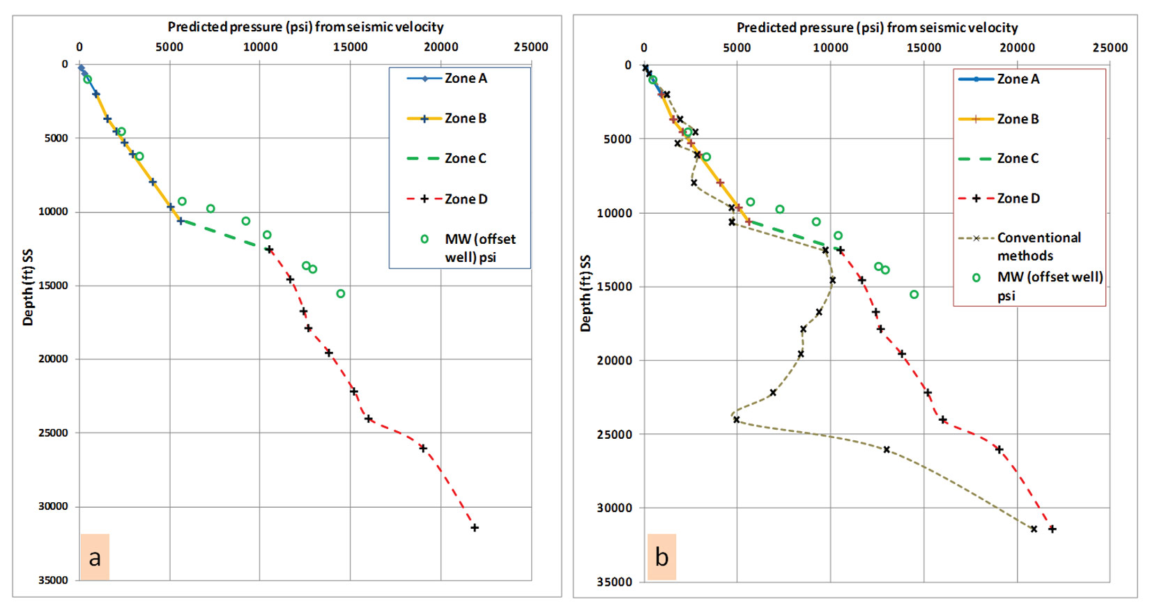
The new proposed method predicts pressure in each of the four zones individually. It uses the extrapolated Δt_c from zone B only, rather than from zones A and B combined. Note the dramatic difference between the new proposed predictive model and the conventional methods (Figure 8b). The conventional methods produce ambiguous pressure values at zones B and D. Therefore, swaying and breaking the so called NCT might be needed for calibration. This defeats the whole purpose of creating a prediction model that can be used to forecast pore pressure at a new proposed location in the same basin.

In deep water, the modified Eaton’s (x) exponent can vary from 1 to 3. This is contingent on the age, predominant lithology, and the stress vectors in the local basins especially around the salt domes.

Case Histories

1. Trio’s fulfillment

The majority of oil and gas trapped in clastic sedimentary column requires generation of hydrocarbon associated with rising of in situ pressure. Fluids expel from the deeper part of the basin mainly upward. Retaining the fluids exodus leads to generating excess pressure which is the catalyst of hydrocarbon entrapment where structural or/and stratigraphic traps are accessible.

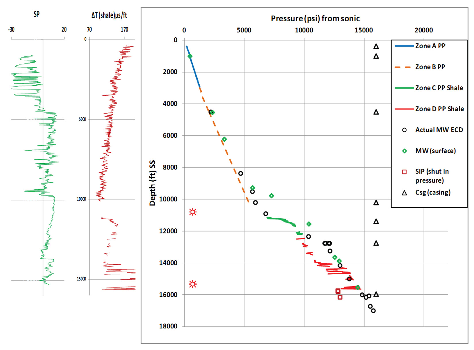
Figure 9 is a classic example of applying the new pressure prediction approach. Thick zone A is due to thick rich sandy section and pressure calculated by applying equation 2. Zone B is predicted by applying equation 9. The pressure ramp (zone C) and the geopressured section below (zone D) are calculated using the horizontal effective stress method (equations 10, 12, and 13). This is a case history where the four zones are well represented and the trio process was consummated. Noteworthily, pay zones in this discovery well are at the top of the pressure ramp and few thin beds within the geopressured section.

2. Geological cause of seal breach

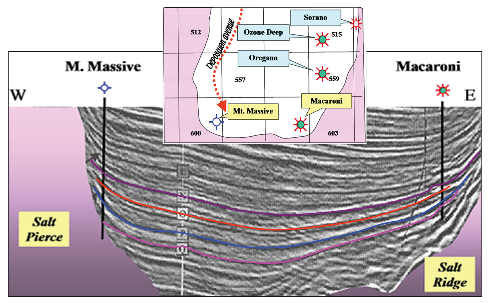
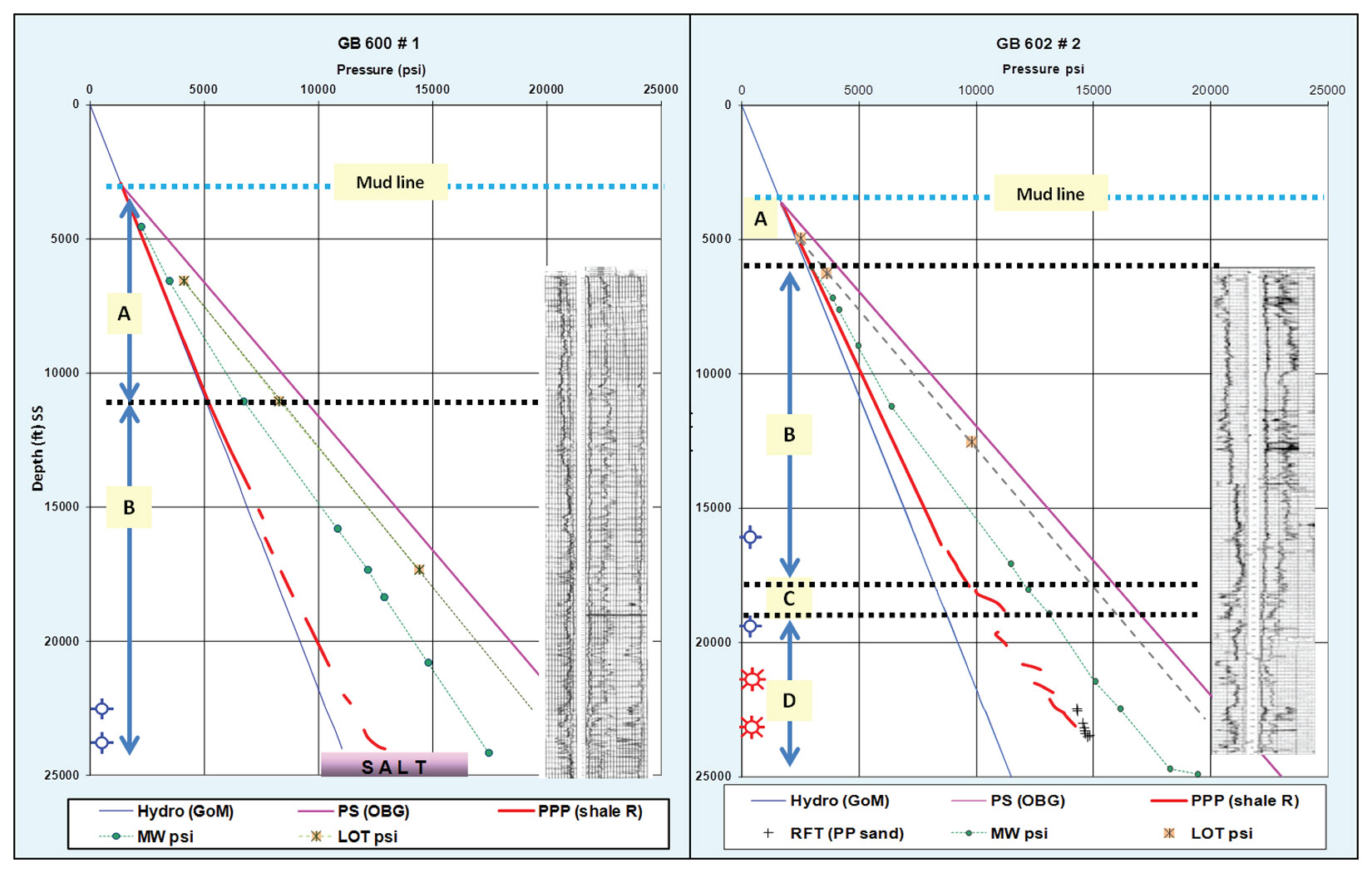
The prolific Auger mini-basin in the Garden Banks area in the Gulf of Mexico (Figure 10) can be used as a classic case history justifying the causes of geopressure, the four subsurface zones, and seal integrity. There are two wells (GB 602 – Macaroni and GB 600 – Mt. Massive) drilled in the same mini salt basin, testing the same stratigraphic sequence on a saddle structure. The wells, drilled on two structural highs at the ends of a saddle, are about 5 miles apart and almost reached the same depth of ~24,000 ft. GB 602 #2 is the discovery well for Macaroni field with a competent seal and well developed geopressure profile (presence of A, B, C, and D zones). On the other hand, GB 600 #1(Mt. Massive prospect) was deemed to be a dry hole with a breached seal and merely bears a hydrostatic and possible hydrodynamic pressure profile (Figure 11).

Examining the geopressure profiles relation and geological setting of the two wells (Figures 10 and 11) sheds light on the pore pressure causes, expulsion and trapping trio concept:

1. The two wells have almost the same depth resulting in equal overburden, the same geothermal gradient and have the same hydrocarbon migration path. This should lead to an equal source of geopressure for both wells, based on the conventional beliefs that stress and heat are the cause of geopressure (excess pressure).
2. The dry hole is in proximity to a sedimentary feeder system. If the concept that a high rate of sedimentation causes pressure surge is correct, the dry hole (GB 600) should have greater pressure than GB 602.
3. Examining both ends of the seismic cross section sheds light on the salt emplacement history. On the field side, sedimentation was contemporaneous with the salt ridge rising. However, on the dry hole side, salt was intrusive (salt pierce) and penetrated the section post sedimentation (Shaker, 2002 and 2004), creating a breaching gouge zone between the sediment and the salt mass interface at the GB 600 prospect.
4. On GB 602 the four geopressure zones are well-developed with a pressure surge of approximate 1500 psi at the pressure ramp (zone C) and the pay zones in zone D. On the other hand, the bottom of zone B on the GB 600 profile can barely be recognized on the breached pressure profile (Figure 11).

This case history demonstrates that geopressure (i.e. abnormal, excess pressure, and overpressure) build-up takes place if the geopressure trilogy process is fulfilled, from generation to expulsion to retention. Zone C presence in the subsurface is a key gauge for risk assessment.

Summary and Recommendations

The newly introduced before drilling prediction method is valid and applicable in most of the Gulf of Mexico with exception of the Florida carbonate platform. The depth range where this method is applicable depends on velocity picks accuracy and spacing. An average depth of 25 kft to 30 kft is reasonably applicable (Figure 2). It can be successfully used in young (Cretaceous to Holocene) clastic sedimentary basins worldwide. This is due the fact that most of the conventional prediction methods were initiated in the Gulf of Mexico.

1. Pressure generation due to stress, heat, dehydration, and fluid expulsion alone do not result in creating overpressure. A retention seal is required to prevent the in situ formation fluids from escaping and fulfilling the trilogy cycle.
2. Defining the four pore pressure zones (A, B, C and D) using seismic velocity is a keystone for any pre-drilling pore pressure prediction.
3. The assumption that the sedimentary section above the top of geopressure (i.e. zones A and B) is hydrostatically (normally) pressured can lead to erroneous pore pressure prediction outcomes.
4. The gradual reduction in porosity during the expulsion phase (zone B only) impacts the petrophysical properties (V, R, ρc, etc.). The power law trend line that connects the data points, in zone B, is called the compaction trend instead of normal compaction trend.
5. Calculating the slope of the CT in zone B is essential for extracting the petrophysical property values (V_c, R_c, ρ_c, etc.) in zones C and D in order to perform a reliable prediction.
6. Empirical depth-pressure relationship should be established to predict pressure in the hydrodynamic zone B instead of considering it as a hydrostatically pressured zone.
7. Effective stress theorem only applies on zone C and D. Therefore, pore pressure should be calculated in zones A and B separately.
8. Integrating the subsurface geology, including any possible structural failures, with petrophysical properties and the proper prediction methods can lead to adequate pore pressure prediction, and avoid high exploration risk and serious drilling hazards.
9. The equations’ constants and exponents introduced in this paper are subject to modification in different basins.

Finally, software is not “one size fits all”. The geological building blocks incorporated with the predictive algorithm methods are the backbone of any pore pressure prediction.

Acknowledgements

The author gratefully acknowledges the conscientiousness of the CSEG RECORDER volunteers, especially Dr. Rob Holt and Dr. Satinder Chopra, for taking the time to review and evaluate the data manuscript. Many thanks are due to Dr. Barry Katz for his editing and technical guidance.