A new, simple approach to surface-consistent scaling

Surface-consistent scaling has been a standard step in the processing of land seismic data for many years, especially in the preparation of pre-stack data for AVO analysis and inversion. Despite the fact that this type of process is in such common use, we believe that there is a basic problem with how the surface-consistent scaling equations are solved in situations where there are surface-consistent variations in noise as well as signal. Since spatial variations in signal-to-noise are observed in most land datasets, we believe that the scaling problem that we address here could be an issue wherever the near-surface conditions generate large variations in signal-to-noise ratio in the seismic survey. This is true for many Canadian seismic datasets because of all the recent glacial and inter-glacial periods of erosion.

Experienced land seismic data processors know that the scalars derived by the surface-consistent scaling process can be highly influenced by noise. So it is common to try to design the surface-consistent scalars on data that contain the best signal-to-noise ratio possible in a similar fashion to other surface-consistent processes like statics and deconvolution. This means that the data being used for deriving the scalars will often be a noise attenuated and frequency band-limited version of the data that the scalars are actually applied to. These noise attenuation steps do help to provide scalars that are better derived from signal rather than noise. However, the need for the new approach to scaling presented here was motivated by the observation of many datasets that suffered from obvious scaling problems, even after great care was taken to derive accurate surface-consistent scalars.

It is only relatively recently (perhaps in the last 10 years) that there has been a requirement for the majority of land seismic datasets to be processed in a fully AVO-compliant manner. We believe that this explains why this issue with the surface-consistent scaling algorithm has not been fully realized before now.

The scaling problem that we have frequently encountered typically manifests itself by a decrease in the amplitude of the reflections in noisy parts of the stacked volume compared to less noisy sections. We point out in this article that there is a very simple reason for this: the influence of the noise on the measured trace amplitudes is always additive, surface-consistent scaling is designed to balance the total amplitude of the traces, therefore, after scaling, the level of the signal always goes down as the level of the noise increases. In the language of statistical analysis, we are using a biased estimate of the signal amplitude. The trace scalars that we obtain by normal surface-consistent scaling are typically too small because our basic amplitude measurement is the amplitude of signal plus the amplitude of noise. The noise attenuation steps referred to in the previous paragraph would have to succeed in attenuating the noise perfectly in order to obtain the correct scalars.

Residual source and receiver-consistent scaling problems can be difficult to notice and hard to recognize on CDP stacks. However, the problem can be very clearly seen on source and receiver stacks as vertical bands of hot and cold amplitudes.

We suggest a simple alternative method of surface-consistent scaling that is based on measuring unbiased estimates of source and receiver- consistent scalars from source and receiver stacks. In order to reduce the effect of CDP structure on the surface-stack amplitudes, the data need to be flattened within the analysis time window before stacking, so our approach is only appropriate for relatively simple geologic situations where this is possible. In addition the average amplitude variation with offset within the time window needs to be removed before forming surface stacks. We expect that our method could be used effectively in most of the onshore unconventional play areas in Canada and the United States that are currently attracting interest.

In this article we begin by showing evidence of incorrect amplitude scaling of the seismic signal on a real data example after the normal surface-consistent scaling process has been applied. An explanation for the poor scaling is then proposed with the aid of synthetic data that includes both surface-consistent signal and surface-consistent noise. Finally, a simple unbiased method for solving the surface-consistent scaling equations is proposed.

Real data example of the problem

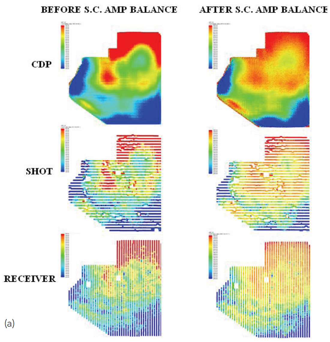
We start with an illustration of the scaling problem on real data. Fig. 1(a) shows a central inline from a CDP volume of land 3D data that has been processed in a fully AVO-compliant manner so that the amplitudes and phase of signal (the reflections) are preserved as much as possible while attenuating the various types of noise. It has undergone fully surface-consistent processing with refraction statics, residual statics, amplitude scaling and deconvolution all being done in a surface-consistent manner.

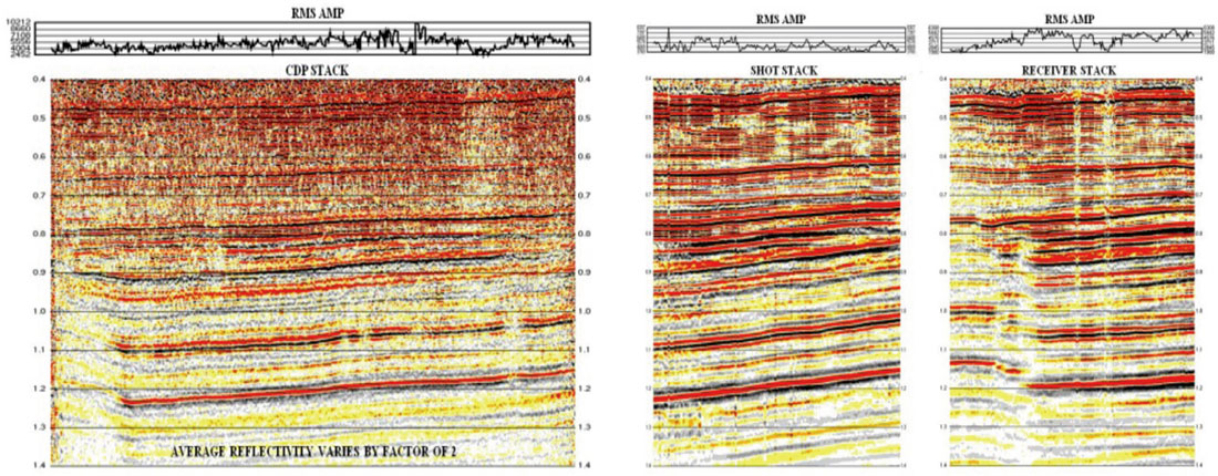
On the top of the section is plotted the RMS amplitude of the bandpass filtered CDP stacked traces. The amplitudes are calculated within a time window where the signal is strongest. The RMS amplitudes vary along this inline by more than a factor of two, which seems somewhat large since this implies that the average reflectivity of the Earth within the RMS amplitude time window varies laterally by this amount. However, this amount of amplitude variation on CDP stacks of land data after AVO-compliant processing is often observed, so this observation alone may not warrant much concern.

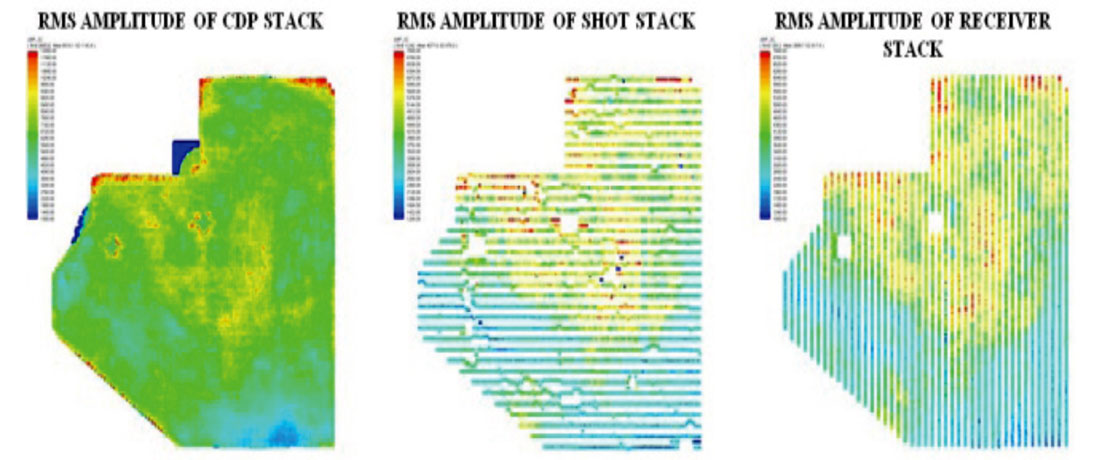
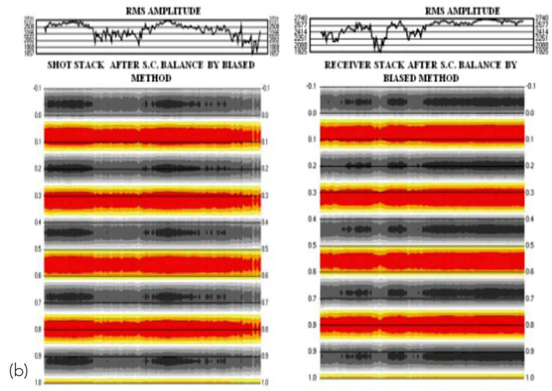
When we examine the RMS amplitudes of the shot and receiver stacked traces in Fig. 1(b) however, we see vertical banding due to high-amplitude and low-amplitude variations from shot-to-shot and receiver-to-receiver, which are also indicated by the RMS amplitudes plotted above the traces. When we look at a map view of the RMS amplitudes of the CDP, shot and receiver stacks in Fig. 2, we can see an obvious similarity between the surface locations of the RMS amplitude variations on all three stacks. The RMS amplitudes of the shot and receiver stacks vary by more than a factor of four around the 3D survey. Since the purpose of surface-consistent scaling is to remove this type of shot-to-shot and receiver-to-receiver amplitude variations, it certainly appears as if surface-consistent scaling is not correctly balancing the amplitudes in the data.

This dataset is not unusual in the way the surface-consistent scaling has failed to properly balance the amplitudes of the reflections in the data. We have observed similar results on many datasets that have been processed by different processing companies and with different software. In practice, the amplitude variations of the signal on the CDP stacks are so large that a CDP-consistent amplitude correction is used to “compensate” for the problem. This is not appropriate because a non-surface-consistent correction is being used in an attempt to correct for a problem that is really surface-consistent. We believe that this scaling problem has a relatively simple cause and solution, which we will now attempt to explain.

Surface-consistent scaling basics

Surface-consistent scaling is used on land seismic data in order to compensate for the effects of the highly variable near-surface layers and variable source and receiver signatures and coupling. The surface-consistent method was first introduced by Taner et al. (1974) and analysis of the amplitude scaling problem was done by Taner and Koehler (1981), Yu (1985) and Taner et al. (1991).

It is typical to consider that the amplitude of each trace, Aij, from shot i and receiver j is influenced in a multiplicative form by source, receiver, offset and CDP factors respectively:

In order to transform this equation into a linear equation, logarithms of both sides are taken. A set of linear equations is obtained by considering all trace-amplitudes together, and the solution for the four scaling factors is obtained by standard least-squares methods.

There are three well-known ways in which the solution of these equations can go wrong. First, it is assumed that the noise is Gaussian, so large outliers (very high or low amplitude traces) need to be eliminated from the data being analyzed. Second, certain long-wavelength elements of the solution can be poorly resolved (Wiggins et al., 1976). Third, it is known that noise can influence the solution, so it is typical to try to design the correction factors on clean signal as much as possible by applying a bandpass filter, for example, in order to improve the signal-to-noise ratio of the data being used for determination of the scaling correction factors.

In the surface-consistent scaling of the real data example previously shown, great care has been taken to minimize the effect of all of the above three factors that are known to degrade the results. Nonetheless, we still observe the scaling problems illustrated in Fig. 1 and Fig. 2.

Biased and unbiased amplitude estimation

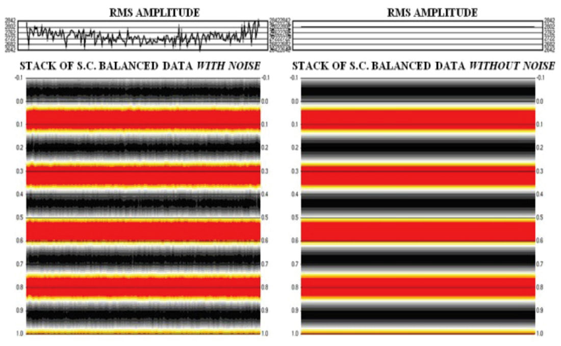
To investigate this issue further, we performed tests on a dataset where the real data traces used earlier in Fig. 1 and Fig. 2 were replaced with very simple synthetic traces without any AVO or structural effects in any direction. Every trace started out identical to all others. A set of shot and receiver-consistent scalars were then applied to these traces by multiplying each trace by the appropriate shot and receiver amplitude factors. Two datasets were formed: one with random noise added and the other without any noise. These datasets were used for first deriving, and then applying, shot and receiver-consistent amplitude scalars.

In short, the surface-consistent scaling results on both the datasets worked perfectly in the sense that the relative differences in amplitudes between shots and receivers were successfully removed. However, one important difference did occur. Fig. 3 shows the CDP stacks of the synthetic datasets with and without noise. Notice that the RMS amplitude of the stacked traces is lower, in general, with random noise compared to the noise-free data.

To understand why this difference in scaling occurs when noise is added, we need to understand how the estimate of the amplitude on each trace is made. The amplitude of a trace is normally estimated by calculating the RMS amplitude within a time window. Suppose there is both signal, s(t), and random noise, n(t), present on each trace. Then,

The inequality holds because the signal and noise are uncorrelated. In terms of expectation values,

where we have used the fact that E{2s(t)n(t)} = 0 for uncorrelated signal and noise. So the measure that is used for estimating the amplitude of the signal on prestack traces is a biased estimate. Hence, the more random noise that is added, the higher the amplitude estimate becomes and the more the signal is erroneously scaled down in amplitude, as in Fig. 3.

It is important to note that RMS amplitudes of the shot and receiver stacked traces are unbiased estimates of the signal amplitude for each shot and receiver (in the absence of offset and structural effects on the amplitudes). This is true because

where we have used the fact that the random noise has a mean of zero.

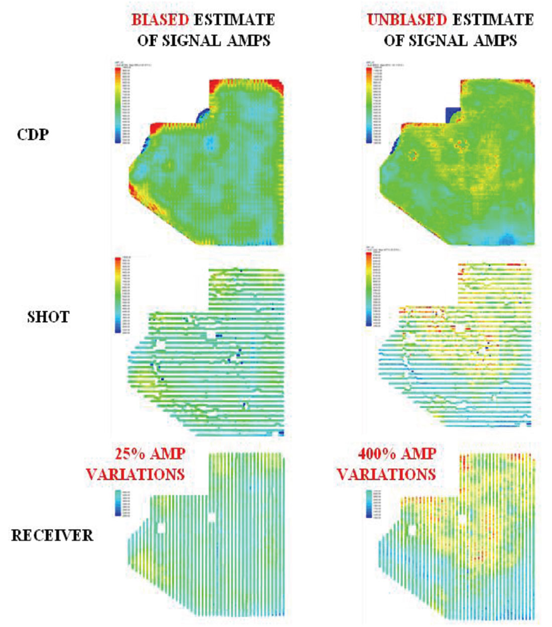
Using a biased measure of amplitudes causes the sum of signal and noise to be balanced when solving Eqn. 1. An unbiased amplitude measure causes just the signal to be balanced. Fig. 4 illustrates this point on the real data by comparing the stack of the RMS amplitudes (the biased estimate) to the RMS amplitudes of the stacks (the unbiased estimate).

Surface-consistent signal and noise

In order to generate the same type of scaling problems on synthetic data that we observe on real data, we need to consider synthetic traces that have both surface-consistent signal and surface-consistent noise. We routinely see the effects on land data of good and bad data areas. Some surface areas generate much more noise due to backscattering, for example, than others. So shots and receivers at those surface locations will have more noise than elsewhere. This would be true even if the amplitude of the signal were perfectly scaled at every shot and receiver location. So we expect noise to be surface-consistent, and furthermore, we expect the surface-consistent scaling factors for the noise to be different from the scaling factors of the signal.

We have generated another set of synthetic traces where each trace D_ij(t) is scaled with different shot and receiver scalars for the signal (S and R) and the noise (Sn and Rn):

Fig. 5(a) shows the RMS amplitudes of the CDP, shot and receiver stacks before and after surface-consistent scaling that is performed in the usual way with the biased amplitude measure. The result is now similar to what we see on real data: the signal amplitudes have changed but they are obviously still poorly balanced. Furthermore, in Fig. 5(b) we see the same type of high and low amplitude banding on the shot and receiver stacks of the synthetic data that we observed on the shot and receiver stacks of the real data in Fig. 1(b).

By performing surface-consistent scaling with a biased amplitude estimator with a model that includes both surface-consistent signal and surface-consistent noise, we have been able to reproduce the same type of amplitude scaling problems that we observe on real data.

An alternative solution

Now that we understand the origin of the problem, we can start to come up with various schemes for overcoming it. The important point is that our normal biased method for estimating signal amplitude needs to be replaced by an unbiased estimate when solving Eqn. (1).

We have already noted that the RMS amplitudes of the shot and receiver stacks are unbiased estimates of signal amplitudes when AVO and time-structure are not complicating factors. As long as the time structure is similar within the analysis time window, it is possible to minimize its effect on surface-stack amplitudes by flattening beforehand. In addition, AVO-effects can be minimized by measuring, and removing, the background AVO variations before stacking. We have found that most datasets that are of interest for AVO analysis and inversion conform to these conditions.

A particularly simple method for solving the surface-consistent scaling equations in an unbiased fashion that works well for data that conforms to these conditions is to use a sequential approach: First estimate the shot scalars from the RMS amplitudes of the shot stacks. Apply the inverse of these shot scalars to the pre-stack traces, and then estimate the receiver scalars from the RMS amplitudes of the receiver stacks. Apply the inverse of these scalars to the pre-stack traces. Repeat these steps until the data are balanced sufficiently. Note that this method (a variation on Gauss-Seidel matric inversion) is analogous to old methods of surface-consistent deconvolution (performing ensemble-deconvolution on shot gathers, then receiver gathers) before more efficient methods came along (Cary and Lorentz, 1993).

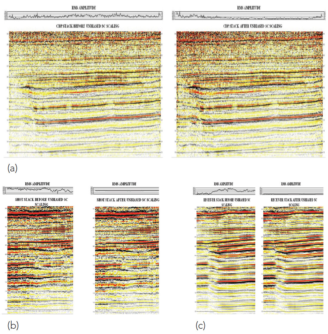
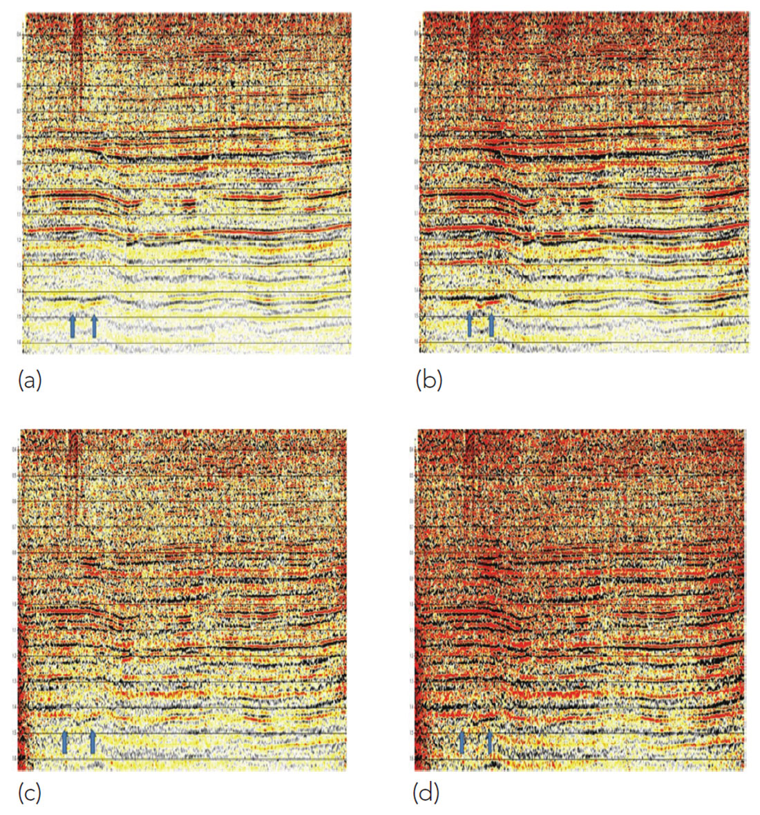
Fig. 6 shows the effect of applying five iterations of this algorithm to the real data example. The amplitudes are better balanced in all domains: CDP, shot and receiver. To understand the potential impact on AVO analysis of biased vs. unbiased surface-consistent scaling, we show in Fig. 7 examples of intercept and gradient calculations along one of the inlines. As expected, high and low amplitude banding is corrected in the data with unbiased scaling.

Conclusions

The main point of this article is remarkably simple. We have shown that the usual method for solving the surface-consistent scaling equations causes the signal plus the noise to be amplitude- balanced. We want to balance just the signal so we need to use an unbiased amplitude measure instead of the biased measure that is normally used. Real and synthetic data examples were used to illustrate the problem and a simple alternative method for solving the surfaceconsistent scaling equations was suggested.

Acknowledgements

We thank Arcis Seismic Solutions, TGS for permission to publish this work. The data example is the Kimiwan 3D from the Arcis Data library.