A Review on Least Squares Prestack Migration and its Applications

Summary

Kirchhoff least squares prestack migration (LSPSM) attenuates acquisition artifacts resulting from irregularities or sparseness in the wavefield sampling and improves image resolution. This paper provides a brief review on the advantages and disadvantages of using LSPSM. Using synthetic examples, a few applications of LSPSM including improvement in image resolution, the ability for data reconstruction, velocity evaluation, migration velocity analysis of incomplete data, and its application for time lapse seismic imaging is shown. The disadvantages of the method are also briefly discussed throughout the paper.

Introduction

Kirchhoff seismic modeling or de-migration is an example of operators that can be written in terms of a linear problem in the general form of

where d is the observed seismic data, m is the earth reflectivity model, and G is the Kirchhoff seismic modeling operator which contains diffraction shape and wavelet information (Yousefzadeh and Bancroft 2012a,b). The inverse process,

recovers the earth model or reflectivity from the seismic data. The number of entries in G is equal to the number of grids in the model domain multiplied by the number of observations. Since the matrix G is not square and is extremely large, calculating the direct inverse of G is impractical. Thus, approximations to the inverse are used instead. A common approximation uses the adjoint (mathematical transpose) of G given by

where m̂ is the migrated image and G^T is the Kirchhoff prestack migration operator.

Because of its many advantages, Kirchhoff migration remains one of the main practical choices for migration of seismic data. Its ability to handle incomplete and irregularly sampled seismic data is a main advantage of Kirchhoff migration over other migration methods. However, incomplete data produces migration artifacts and gives a blurred image of the subsurface reflectivity. LSPSM is less sensitive to the data irregularities and is able to reduce the acquisition footprint and produce a high resolution image (Nemeth et al., 1999). In the method of LSPSM, migration artifacts are attenuated by minimizing the difference between the observed data, d, and the modeled data, Gm̃, expressed by | Gm̃ – d |, where m̃ is an approximation to m (Nemeth et al., 1999).

The first term on the right hand side of equation 4 is the data misfit. In the minimization of J(m̃), this term recovers a model to fit the data. The second term is a regularization term that serves to emphasis or attenuates models with certain features and µ is the regularization weight. The minimum or Euclidian norm is the simplest form of the regularization function,

which leads to the stable damped least squares solution, m_DLSM , to the problem and is given by

where I is an identity matrix.

The matrix G^T G is a square matrix and is invertible. However, it is a very large and dense matrix (Yousefzadeh and Bancroft 2010). Therefore, LSPSM is an expensive procedure and solving equation (5) requires an iterative method such as Conjugate Gradients (CG) (Hestenes and Steifel, 1952) or a modified version of that, Least Squares Conjugate Gradients (LSCG) (Scales, 1987). Each iteration of the LSCG is at least two times more expensive than the conventional Kirchhoff migration of the same seismic data. In addition to high cost, LSPSM requires an accurate estimation of the background velocity. Without a reasonably accurate velocity, LSCG method to solve LSPSM equation does not converge to a high resolution image. LSPSM is more sensitive to the accuracy of the velocity information than the conventional Kirchhoff migration (Yousefzadeh, et al., 2011 and 2012). Five applications of LSPSM are briefly reviewed in the following.

1. Kirchhoff LSPSM for image resolution

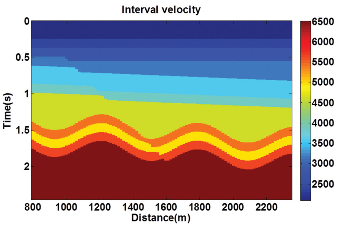
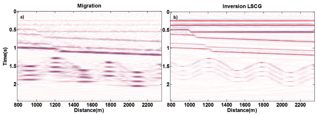
To show the advantage of LSPSM, consider an acquisition geometry with 16 sources and 96 receivers per source. The source interval is 187.5m and the receiver interval is kept at 15.625m to keep the fold number at 4 on a 3km 2D velocity model. This geometry is considered on an earth model with horizontal and faulted dipping and folded layers as shown in Figure 1. Synthetic data are generated and 1% random noise is added to the data. Peak amplitude of noise is 1% of peak amplitude of data. Subsequently, the data are decimated by randomly eliminating 80% of the traces. The Conventional Kirchhoff migration of the decimated data is shown in Figure 2a. Applying the LSPSM to the decimated data creates the image in Figure 2b in which most of the migration artifacts in Figure 2a are attenuated. The LSPSM produced an image with higher resolution than the conventional Kirchhoff migration. The fault, shallower reflectors, and structures are better resolved using LSPSM. Comparison between migration and LSPSM can also be quantified by measuring the relative magnitude of the reflectivites in the corresponding final migration and LSPSM images and comparing them with the true reflectivity model as shown by Yousefzadeh (2012).

2. LSPSM for data reconstruction

LSPSM can also be used for data interpolation. There are many processes in seismic data analysis which require regularly sampled data. Some methods of multiple attenuation and migration in the frequency domain require regularly sampled data. Nemeth et al. (1999) suggested data reconstruction and interpolation using LSPSM. Since the resulting image of LSPSM is a high resolution image, it can be used in a forward problem to reconstruct data with a desired geometry. Suppose G_i and d_i represent the forward modeling operator for the incomplete data, and incomplete data respectively. The damped least squares image is computed by solving

equation. The regularized data, d, can be generated by forward modeling of m_DLS and is given by

This method of data reconstruction is robust. However, it is more expensive than the other interpolation methods which usually use properties of the Fourier transform and work with a small part of the data (one shotgather for instance) at a time. For data

reconstruction by LSPSM, LSPSM images must be computed. This is an expensive and time consuming procedure. Adding to this cost, an additional cost of forward modeling of the LSPSM image with the new geometry of source and receivers, gives the total cost of data reconstruction by LSPSM.

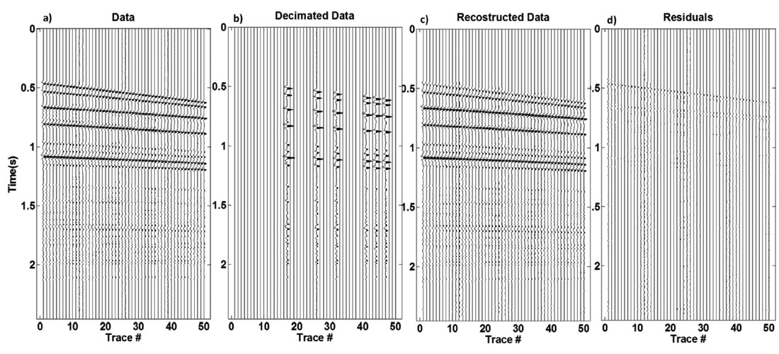
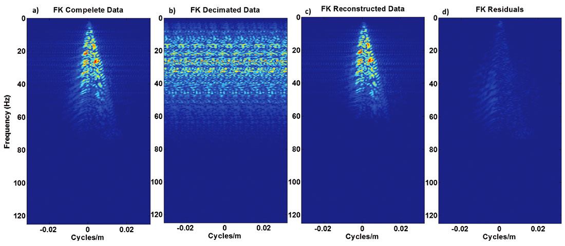
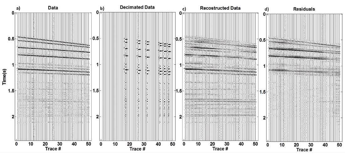
To show the ability of data reconstruction with LSPSM method, the LSPSM image in Figure 2b is used for data reconstruction when 80% of data are randomly decimated. Results for the first 50 traces in a shotgather are shown in Figure 3. Panels a, b, c, and d in Figure 3 show the original, decimated, reconstructed, and residual (difference between original and reconstructed) data, respectively. With having only 20% of randomly selected data, LSPSM is a powerful method to reconstruct the missing traces. Figure 4 compares the FK spectrum of the original, decimated, and reconstructed data, and their residuals. As seen, the decimated data is highly aliased where reconstruction has removed the aliasing effects. Residuals show that the data reconstruction procedure is able to reconstruct frequencies and wave numbers of the original data.

3. Kirchhoff LSPSM for velocity evaluation

Ignoring the high cost, LSPSM is an effective tool for resolution enhancement and data reconstruction. However, its high dependency on the accuracy of background velocity model information is a disadvantage of the method. Using synthetic examples, we show how minor errors in the velocity information lead to major failures in the LSPSM resolution improvement, LSCG convergence, and the data reconstruction. A small perturbation from the true velocity prevents the method from improving the image resolution and correct data reconstruction. Despite these shortcomings, the high sensitivity of LSPSM to the accuracy of the velocity information makes it a practical tool for measuring the accuracy of the velocity model or for updating an estimated model of velocity.

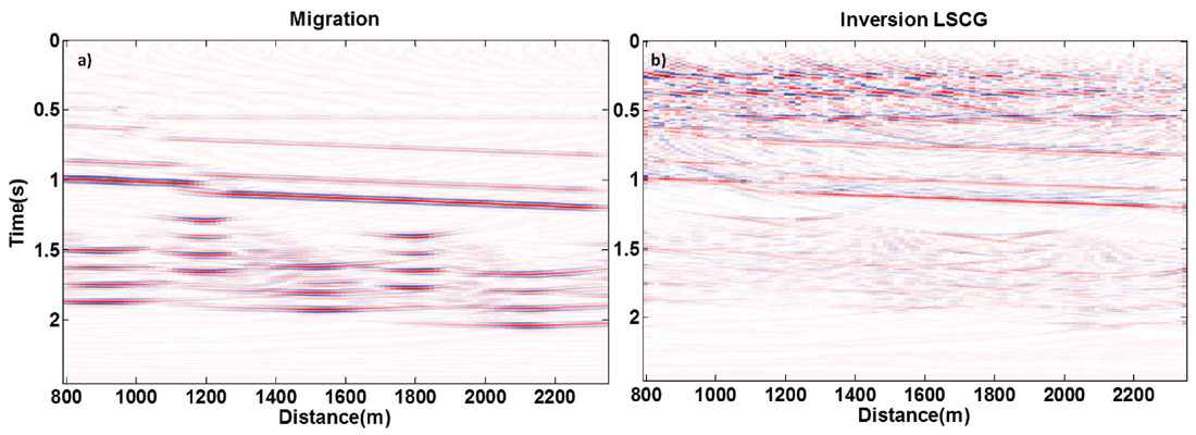
The decimated data in previous example are migrated using conventional prestack Kirchhoff migration (Figure 5a) and inverted using least squares prestack Kirchhoff migration with 20 LSCG iterations (Figure 5b) using a velocity model that is 5% higher than the true velocity. A visual comparison between the two images shows that implementing LSPSM method has improved the temporal resolution of the conventional migration due to act of its intrinsic least squares deconvolution operator. However, it has degraded the spatial resolution and introduced more noise.

The LSPSM image in Figure 5b is calculated with 20 iterations in LSCG. The convergence rate in the LSCG method is an appropriate way of measuring the ability of the LSPSM method in finding the best reflectivity image. In this study, the convergence rate is the relative Euclidean norm of the difference between the original data and the data achieved by forward modeling of the LSPSM image after each iteration. Figure 6 shows the convergence rate when true, higher, and lower velocities of 5%, 10%, and 20% are used. The residuals converge to 4% in 20 iterations when using the true velocity, but will not be less than 42% with 5% higher or lower velocities and less than 83% with 20% higher or lower velocities. Due to the sensitivity of the LSPSM method to the velocity accuracy, small inaccuracies in the velocity information significantly reduce the LSCG convergence rate. With real datasets using a reliable velocity model, convergence rate may be three times slower than this synthetic example. However, with inaccurate velocity information real data may not converge to less than 90% in 20 LSCG iterations.

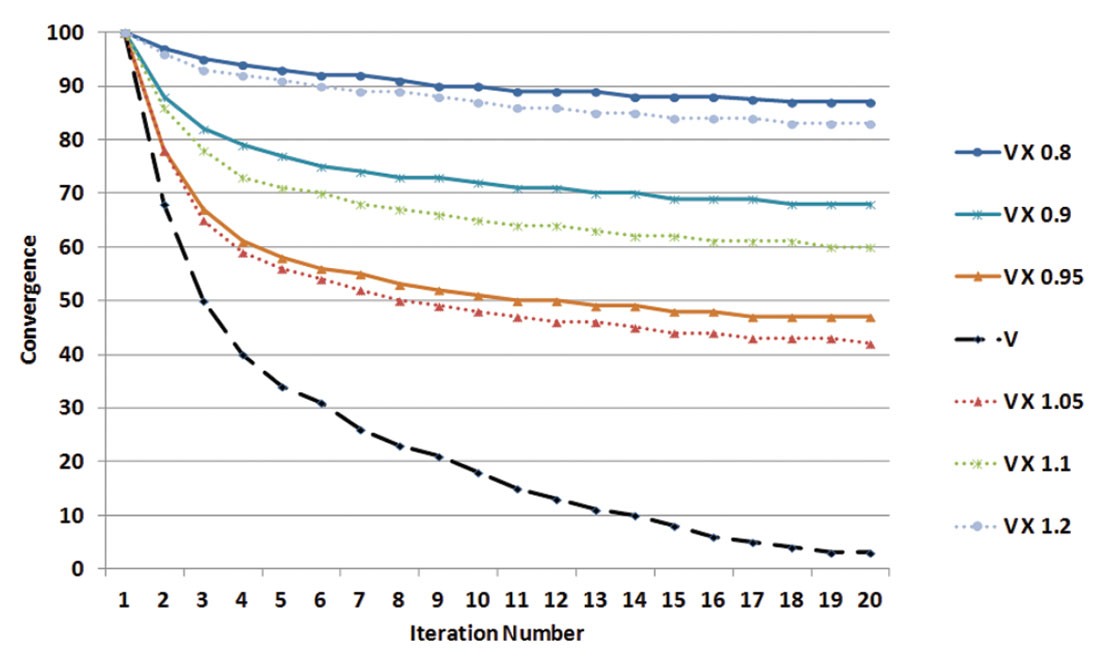
Figure 7 shows the data reconstruction with LSPSM when the implemented velocity is 5% higher than the true velocity model, where panels a, b, c, and d show the original, decimated, reconstructed, and residual data, respectively. The high amplitudes of the residuals in Figure 7d shows the data reconstruction fails when using only 5% higher values than the true velocity.

The image resolution improvement, data reconstruction, and LSCG convergence rate are three factors which can be used for the evaluation of the accuracy of an imaging velocity model. The best velocity model is the model that improves the conventional migration resolution by LSPSM, gives less residual energy in data reconstruction, and better convergence rate in LSCG method (Yousefzadeh and Bancroft, 2012d). For instance, with a real dataset, one can remove some traces and then using the proposed method and with a range of estimated velocities, perform data reconstruction. The velocity model that gives the lowest residual and better convergence rate is probably the best velocity to be used for imaging.

4. Kirchhoff LSPSM for velocity analysis of very sparsely sampled data

As shown in the previous section, LSPSM, which does not require dense and regularly sampled data, is very sensitive to the accuracy of the velocity model. These properties make it a practical choice for migration velocity analysis of irregularly and sparsely sampled seismic data.

Yousefzadeh et al. (2012) showed that the Common Image Gather (CIG)s from LSPSM have higher resolution than the conventional migration CIGs, especially in the shallower parts of the gathers. The higher resolution image of offset domain CIGs resulted from LSPSM compare to conventional migration CIGs image makes LSPSM CIGs a practical choice for velocity analysis of irregular and sparse data by the semblance method. Yousefzadeh et al. (2012) extended the migration velocity analysis on migration offset domain and shot domain CIGs to the corresponding LSPSM CIGs. They showed that using unnormalized cross-correlation sum for measuring the coherencies in the shot domain CIGs provides velocity information that is accurate enough to improve the image resolution via LSPSM and give a good data reconstruction result (Yousefzadeh, et al., 2011).

5. Kirchhoff LSPSM/Inversion of time lapse data

Ignoring differences in acquisition instruments, environmental noise, and processing flows and parameters, monitor surveys must exactly follow the baseline survey geometry. This is not always feasible in land seismic and almost impossible in marine seismic acquisition using streamers. An example is the failure of a geophone that has been cemented in a fixed location. Different acquisition geometries leave different patterns of acquisition footprint in baseline and monitor survey migration images. Consequently, the resulted time lapse image show unreal changes in the model parameters in the reservoir rocks.

In 4D seismic studies, LSPSM can reduce matching problems by producing images which are less sensitive to the geometries of baseline and monitor surveys. The data reconstruction ability of LSPSM also makes the baseline and monitor datasets comparable by reconstructing data for both surveys in a new geometry (Yousefzadeh and Bancroft, 2012c).

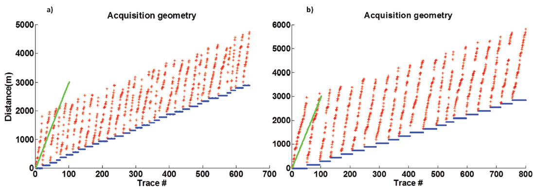
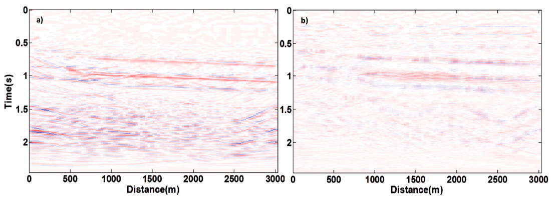
As an example, consider two different seismic survey geometries in Figure 8. The baseline survey includes 32 sources with 100m source spacing, and 100 receivers per shot, with 18m spacing. The monitor survey includes 20 sources, with 150m source spacing, and 200 receivers per shot, with 15m spacing. Both surveys are decimated by removing 80% of the traces randomly. The data for both surveys were migrated and inverted using LSPSM for comparison. Figure 9a shows the difference between the two conventional migration images and Figure 9b shows the difference between the two LSPSM images, as the time lapse images. Since there is not any change in the velocity (and reflectivity) model, that differences must be zero. However, due to the difference in data acquisition parameters, migration images from baseline and monitor surveys have different acquisition footprints. Therefore, the time lapse image shows changes which are not due to change in the model parameters as seen in Figure 9a. However, as seen in Figure 9b most of the artifacts are attenuated in the LSPSM time lapse image.

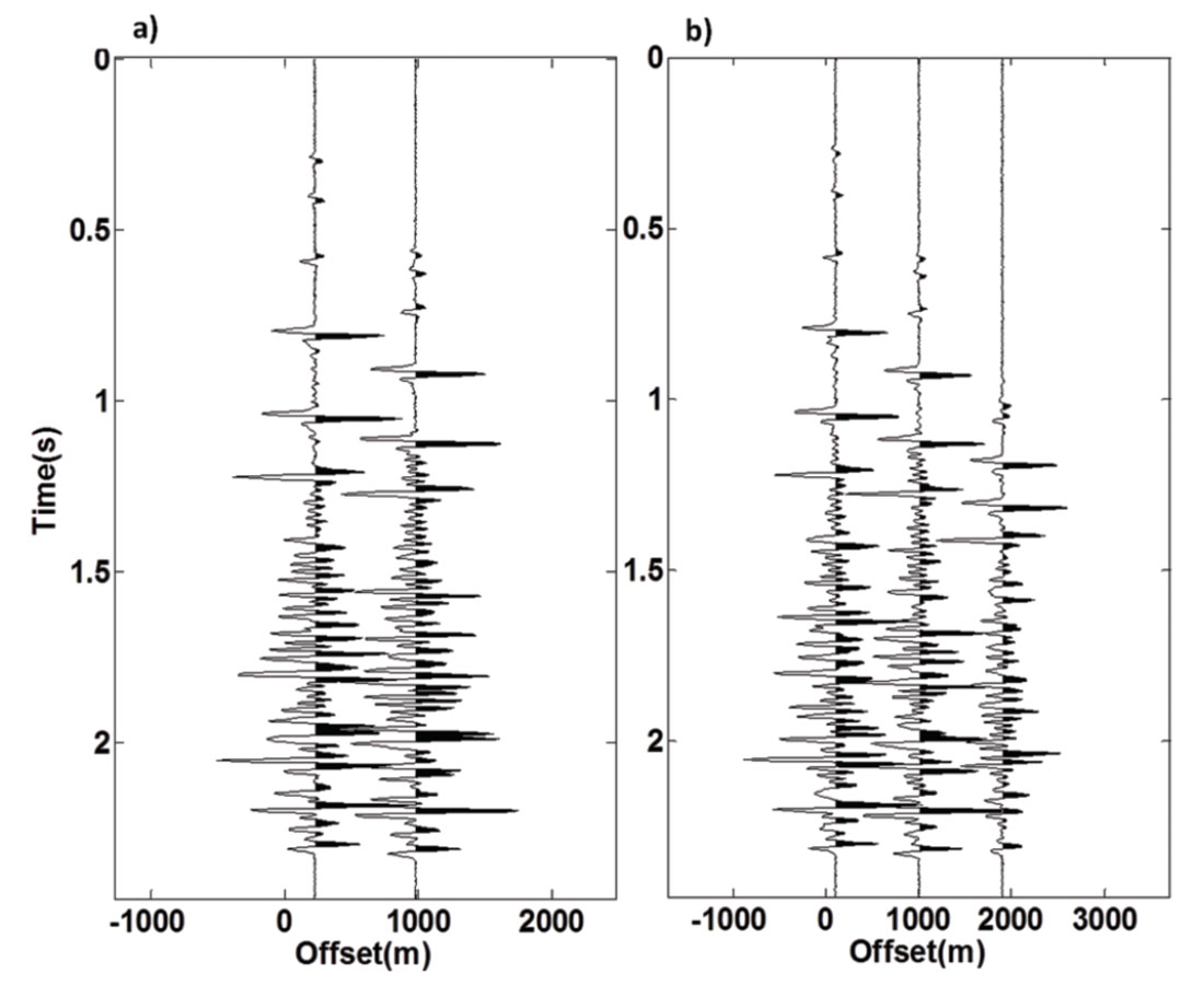
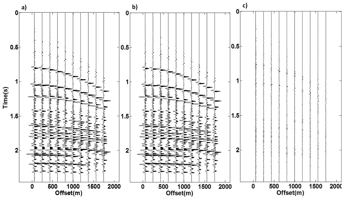
The data reconstruction ability of LSPSM facilitates prestack time lapse studies by generating comparable data for both baseline and monitor surveys. This is achievable by forward modeling of the separate LSPSM images of baseline and monitor surveys with a new geometry. Figure 10 shows the data from the baseline (a) and monitor (b) surveys for a CMP that is positioned at the middle of the seismic line. The comparison is not feasible since the traces have different offsets. Figure 11 shows the reconstructed data from the baseline (a) and monitor (b) surveys. Comparison between these two datasets becomes possible and Figure 11c shows the difference between the two datasets. LSPSM increases the reliability of time lapse studies by reducing the effects of different geometries of baseline and monitor surveys and reconstructing data which makes the prestack time lapse studies feasible. Joint LSPSM/inversion of time lapse data provides time lapse images which are high resolution and less affected by the different data acquisition geometries of the baseline and monitor surveys (Yousefzadeh and Bancroft, 2012c). Minimizing this cost function of a time lapse joint inversion is an expensive procedure since each iteration of LSCG is at least four times more expensive than one time conventional migration of same data. Solving this joint inversion cost function using LSCG requires more than 20 iterations. However, joint inversion is able to produce higher resolution time lapse images than the separate inversions of the same data.

Conclusions

LSPSM is an effective method to attenuate acquisition footprint and reduce migration artifacts. High resolution images achieved by this method can be forward modeled to reconstruct the data. This method is relatively expensive and requires a good estimation of the velocity. With a synthetic example it is shown how small inaccuracies in the velocity information lead to poor resolution in the LSPSM image. High sensitivity of the LSPSM to the accuracy of the subsurface velocity can be used as a tool for measuring the accuracy of the estimated velocity. Velocity analysis on the LSPSM shot domain CIGs give a velocity that is accurate enough to enhance migration image resolution and perform acceptable data reconstruction. The resolution enhancement and data reconstruction abilities of LSPSM can be used in time lapse seismic studies when the baseline and monitor surveys have different geometries. This is applicable especially in marine streamer data when there is a poor control on the positioning of receivers.

Acknowledgements

Authors wish to acknowledge the sponsors of CREWES project for their continuing support. They express their appreciation to Helen Isaac, Kevin Hall, and Rolf Maier in the CREWES project. We also would like to thank David Cho for his careful review.