A simple way to speed up wave equation migration: using a time-shift imaging condition

Abstract

This article describes a way to speed up downward continuation wave equation migration (WEM) by 200% to 400%, or more, via modification of the conventional imaging condition. Specifically, I introduce a new ‘time-shift’ imaging condition, which can be used to estimate the migrated image in between actual migration depth steps. The technique can be easily used for 2D and 3D prestack common shot downward continuation WEM without significant loss of accuracy. The idea is applicable to poststack migration as well.

Introduction

WEM has many desirable qualities as it solves the wave equation directly, and therefore implicitly carries all natural attributes of wave propagation. This is in contrast to the Kirchhoff migration technique, which requires a lot of explicit programming craftsmanship in order to properly emulate the natural aspects of wave propagation (e.g. summation weights, operator anti-aliasing, handling multi-pathing of wave propagation ...etc.) Furthermore, WEM does not carry the restrictive asymptotic assumptions inherent in Kirchhoff migration (i.e., high frequency and far field assumptions), so it behaves well under a broader set of circumstances. The spatial sampling requirements are about identical to Kirchhoff. However, there are two drawbacks with WEM: first, it is less flexible in output data handling than Kirchhoff, and second, though WEM is highly accurate, it runs several times slower than Kirchhoff under the same resource environment. Addressing this latter drawback constitutes the focus of this paper.

In migration, the zero time-shift imaging condition has been commonly used in order to estimate a migrated image at a particular depth step. Recent variations, namely variable space and time shift imaging methods, have been used for depth-focusing analysis (DFA) for migration velocity analysis (MacKay and Abma, 1992) and for amplitude-versus-angle (AVA) analysis after angle transformation in wave-equation imaging (Sava and Fomel, 2006).

Here, a new, simple and fast application of the variable timeshift (or time lag) imaging condition is proposed to interpolate migration output between depth steps during the downward continuation process. For a typical production application, the downward continuation depth step size Δz is set equal to the depth sampling interval dz (5 m to 15 m), depending on the frequency and complexity of the data, so that the output Nyquist sampling principle will not be violated. In the interest of computational efficiency, it would be desirable to increase the migration depth step beyond the depth sampling interval (i.e. Δz > dz) and to rely on an interpolation scheme to fill in the migrated image at the missing depth steps. The resulting speed increase would be about equal to the ratio between depth step and depth sampling interval (i.e. Δz / dz), although it must be noted that an excessively coarse choice of depth step would not properly handle large velocity variation unless certain corrective measures were made (Mi and Margrave, 2001). In order to gain speed, they employed an alternative approach to interpolation in between depth steps by applying a static phase shift to the wavefields followed by zero time-shift imaging. Later, Fu (2004) attempted to achieve the result by absorbing the interpolation and imaging all at one go. However, my technique provides a more flexible and much faster way to interpolate the image especially when the depth step increases in size. In this paper, the interpolation is performed right at the imaging condition stage rather than either before or after the imaging condition.

This paper is an expansion of my previous paper (Ng, 2007) presented at the 77th SEG annual meeting.

Methods

The foundation for the common shot WEM imaging condition used in this paper is a scaled time cross-correlation (i.e. deconvolution) between the upward propagating receiver data wavefield and the downward propagating source wavefield (Kelly and Ren, 2003). At depth z₁ and lateral position x, its frequency domain expression in 2D is

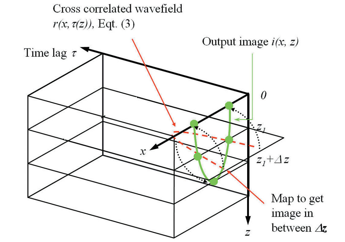
where U(x, z1, ω) is the receiver data wavefield extrapolated to that depth level, and D(x, z1, ω) is the source wavefield extrapolated to the same depth level; ε is a small stabilizing pre-whitening scalar (a tiny percentage of the total energy of the source D), and * denotes the complex conjugate. The standard imaging condition entails computing the zero time (lag τ = 0) cross-correlation by summing R along all frequencies ω in order to estimate an image i(x,z₁). In such case, there is no image output in between depth steps unless a post-imaging interpolation (i.e., up-sampling) is applied to the image i(x,z). But in this paper, instead of summing R along all frequencies, full inverse Fourier transforms are applied to R for every depth step in order to obtain the ‘cross-correlated’ wavefield r(x,τ(z)) at all time lags:

where I have explicitly emphasized the fact that time lag τ will depend on z in the work below. As shown in figure 1, the output image i(x,z) at arbitrary depth z in the vicinity of z₁ is extracted from r between depth steps using the time lag of

where ν is the interval velocity. Further to my previous work (2007), β is introduced as an empirical constant between 0.5 to 1 in order to optimize a range of dips from steeply dipping data to flat data respectively. Generally, β = .75 is recommended. The choice of time lag in equation (3) simulates different coincidence times between the receiver and source wavefields that would be observed at different depths. For z = z₁ (or β = 0), equation (2) will degenerate to the conventional zero time (lag) imaging r(x,τ(z₁)=0) = i(x,z₁). The wavefield extrapolator can be of any type, and here a phase shift plus interpolation (PSPI) with thinlens correction (i.e. extended split-step or phase screen) is used.

Example 1: Impulse response test

The objective of this example is to show how the quality of the impulse responses computed using the time-shift imaging condition interpolation method varies with respect to various downward continuation depth steps (Δz = 10 m, 20 m, and 40 m, which are one time, two times and four times the depth sampling interval dz of 10 m respectively). The velocity used is 5000 m/s, and the CDP interval dx is 15 m. The input impulse maximum frequency is 75 Hz.

Figure 2 shows the ideal reference impulse responses of the shot migration where no interpolation is needed (the migration depth step equals the depth sampling interval, Δz = 1dz =10 m).

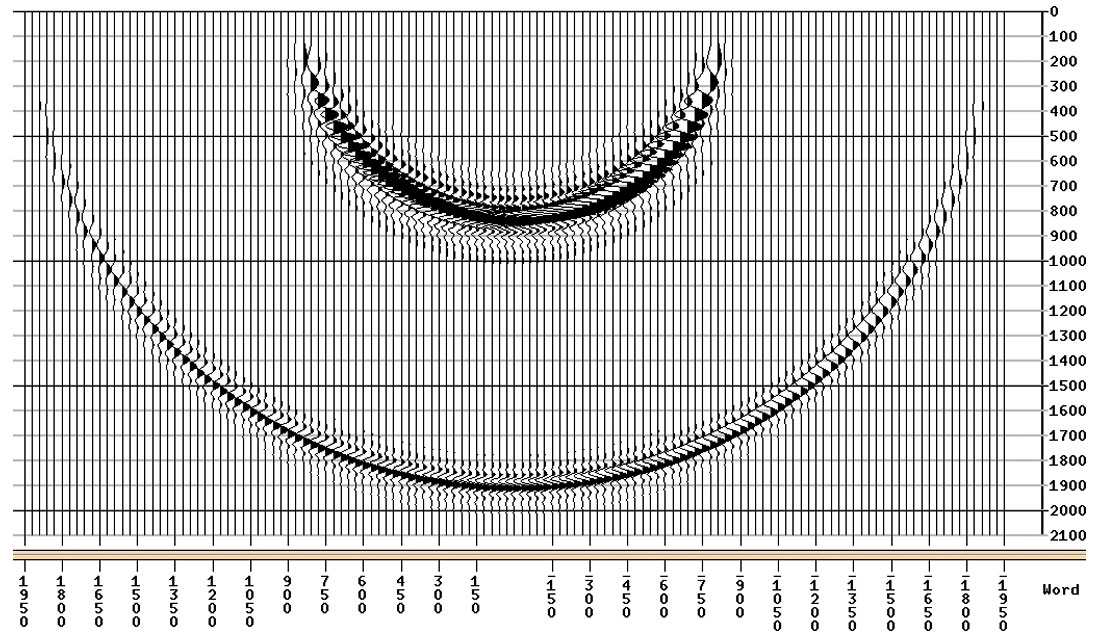
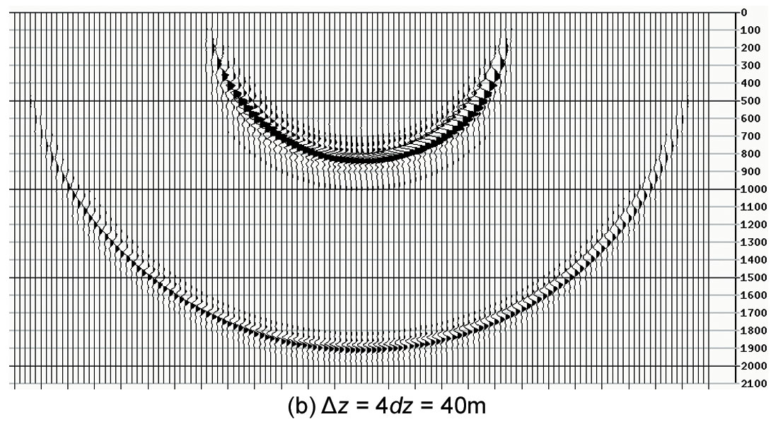
Figure 3 is the shot migration result using post-imaging linear interpolation (i.e., up-sampling) in the depth domain. As the migration depth step increases in size, the impulse responses become increasingly degraded. The result in (a) with a depth step Δz of 20 m (i.e., twice the depth sampling interval) shows a minor degradation and is quite comparable to figure 2. But the result in (b) with a depth step Δz of 40 m (i.e., four times the depth sampling interval) is very poor.

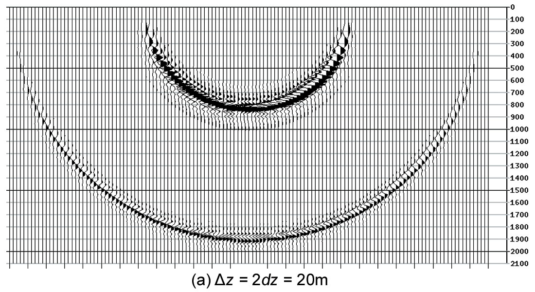
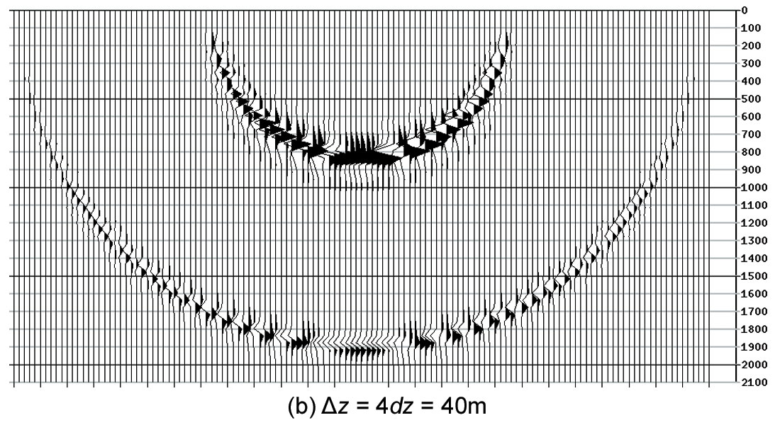
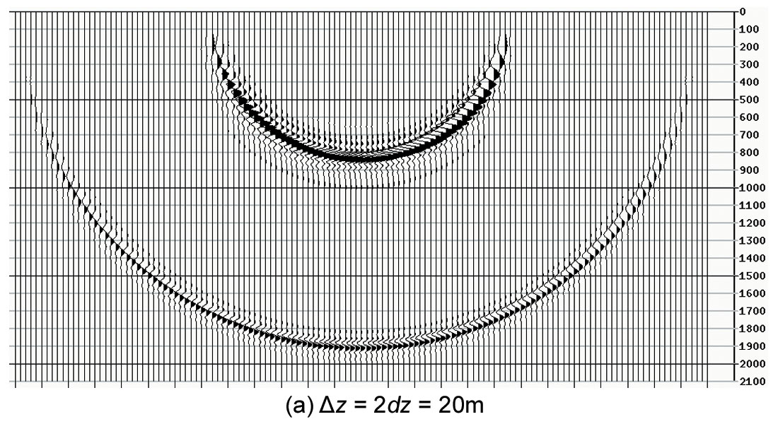
Figure 4 is the shot migration result using the new time-shift imaging condition as the interpolator. The result in (a) with a depth step Δz of 20 m (i.e., twice the depth sampling interval) shows virtually no degradation when compared to the reference figure 2. Even in (b) with a depth step Δz of 40 m (i.e., four times the depth sampling interval), where three interpolated images are output in between actual migration depth steps, the result is very satisfactory showing only minor degradation. The run time is shortened by about four times compared to the reference test in figure 2.

Example 2: Marmousi data set

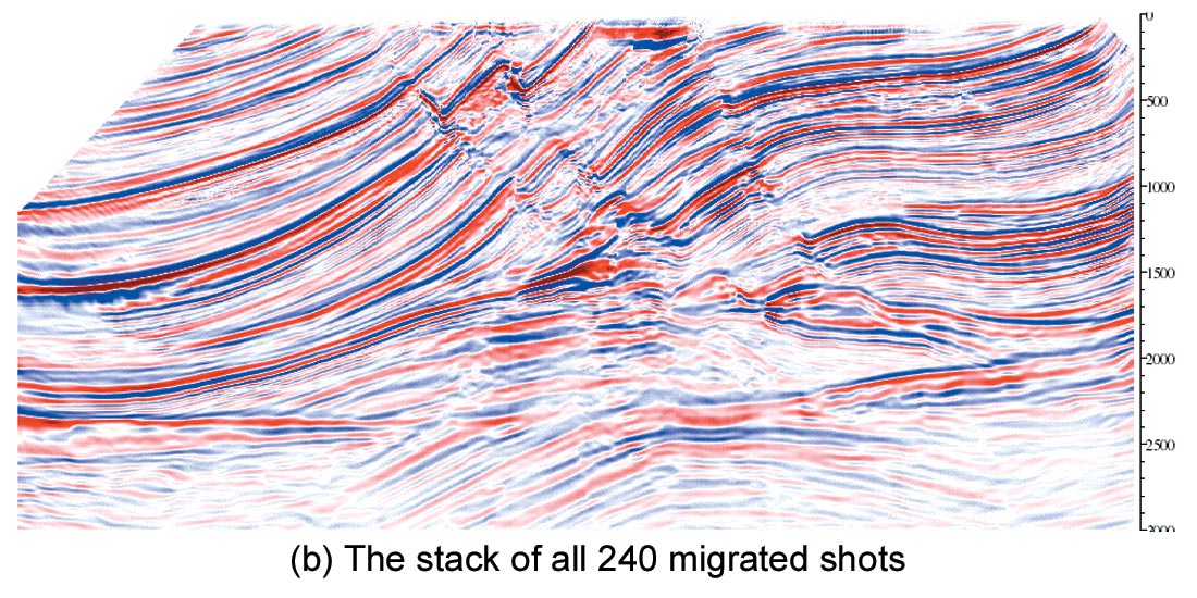
The purpose of this example is to compare the quality of the final stacks between two interpolation methods within the shot migration. One method uses a simple post-imaging linear interpolation, while the other uses the proposed time-shift imaging condition interpolation. In both cases I used a coarse downward continuation depth step Δz of 20 m, which is four times the depth sampling interval dz of 5 m. Five reference velocities are used in each migration depth step of the extended split step Fourier shot migration. The CDP interval dx is 12.5 m. The total number of shots is 240.

Figure 5 is the shot migration reference image (note that interpolation is not needed here as the migration depth step is equal to depth sampling interval: Δz = 1dz =5 m). Note that the dense reflectors in the upper middle section reveal a 30 m wavelength, and according to the Nyquist sampling theorem, simple postimaging interpolation would require a depth step no larger than 15 m (half the wavelength) in order to yield an accurate image.

Figure 6 is the shot migration result using post-imaging linear interpolation in the depth output. A coarse migration depth step Δz of 20 m is used. Note that this depth step exceeds the Nyquist sampling limit of 15 m. As expected, reflectors in most portions of the image show artifacts.

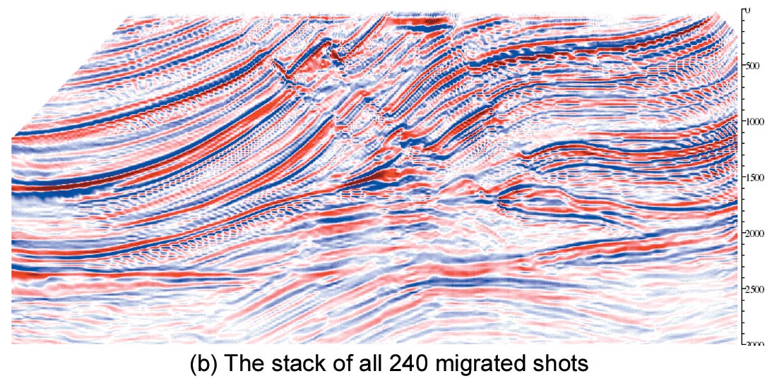
Figure 7 is the shot migration result using the new time-shift imaging condition as the interpolator. The same coarse depth step Δz of 20 m (i.e., four times the depth sampling interval) is used in the migration, but this time the result is quite satisfactory when compared to the reference figure 5, with a very minor loss of resolution. However, the run time is shortened by about four times compared to the reference test in figure 5.

Both figures 6 and 7 reveal some depth errors (less than 0.8% below 2 Km) when compared to the reference figure 5. This is because a coarse migration depth step in heterogeneous media is used, and the velocity field cannot be honored closely. The position error compensation issue associated with using coarse migration depth steps is beyond the scope of this paper but has been corrected by others (Mi and Margrave, 2001).

Discussion of related issues and future work – more questions than answers

Issue 1.

In the future, a better choice of cross-correlation time lags τ may be obtained by incorporating offset information. Specifically, I propose to compute the difference in the direct arrival travel times taken from the shot-to-image-point at depth z and shot-toimage-point at depth z₁, and replace equation (3) by

This will allow an even larger depth step interpolation as it honors the change in the source focusing term where as equation (3) is just a static term instead. The direct arrival travel time imaging in WEM is discussed in Ng (1994).

Issue 2.

Surface topography considerations. Migration algorithms typically use a ‘zero velocity layer’ construct in order to migrate from topography: when the migration depth level is above the surface, use a zero replacement velocity; when the migration depth level is below the surface, use the medium velocity for migration (in particular, I use an implementation described by Reshef (1991)). If the depth step is sufficiently small, there is no need to worry about what to do when the depth level is transitioning through the topographical surface; however, as the depth step increases (in order to gain speed), we have to deal with this issue. Specifically, the conventional ‘all-or-none’ approach zero replacement velocity migration method must be changed to accommodate the surface variations within a migration step.

Issue 3.

What is a good normalization scheme for stacking the migrated shots? This is a general issue related to all shot domain migration methods (a slightly lesser problem exists for offset domain migration methods). After migrating a shot, the output offsets become shot-to-image distances on the surface, not the original input shot-to-geophone distances anymore. Migrated structures would appear in the far shot-to-image offsets in a common image gather (CIG), and consequently normalization for stacking of the CIG can become difficult. How can we preserve the structures’ amplitudes without weakening them during the stacking process (where a set of higher than necessary normalization sample counts is used)? Here, I propose to use a technique similar to the conventional ‘power’ stacking of the data in the CIG’s, weighted by cross correlating it with a ‘model’ trace, which is generated by a simple stack of the original CIG. What needs to be changed is to make the process depth variant.

Conclusions

Due to the fact that time-shift imaging tries to honor the characteristics of wavefield propagation, while the post-imaging interpolation does not, the proposed method produces better results in between depth steps compared to a simple linear interpolation on the post-imaged output.

A time-shift imaging condition can be used as a fast and simple interpolation tool to increase the speed of downward continuation shot migration. The speed increase is about equal to the ratio of the migration depth step size to the depth sampling interval, gaining at least 200% in efficiency.