A Well-Guided Processing Approach

In any processing flow countless parameter choices are made, including which processes to apply, what order to apply them in, and how to parametrize them. In seismic processing, many different but sound choices can all produce similar images. These similar images may not be geologically equivalent when examining all products associated with the creation of the image. Determining which set of choices produces the most geologically accurate and useful result for interpretive work is therefore of utmost importance.

Introduction

“AVO (Amplitude Variation with Offset) friendly” processing or “true amplitude” processing are terms used to describe processing flows that aim to preserve the true AVO trends that exist within a seismic data set. The goal of such processing is to provide a stack and pre-stack gathers that are suitable for interpretation and pre-stack analysis, whether that means the simple derivation of attributes, or the calculation of rock properties through full AVO inversion. As AVO inversion becomes more standard in the interpretation workflow, the need for the early incorporation of geologic information to enhance the quality of pre-stack gathers is essential.

There are many aspects of processing that are inherently interpretive, which is where well-guided processing comes in. It is about using the available geologic information (such as well logs and vertical seismic profiles) from the start through to completion of a processing project, to perform ground truth comparisons. This paper will demonstrate how the use of geologic information throughout the processing flow can provide quality control measures to evaluate amplitude scaling, deconvolution, and velocity analysis, all with the goal of preparing true amplitude data for input into AVO inversion. With the optimization of these stages, it will then be discussed how the use of well-guided velocity volumes can positively impact the inversion workflow.

Deconvolution and Scaling

In an AVO friendly processing sequence, the intent is to preserve the true amplitudes so that the processed data represents reflectivity, while maximizing the bandwidth and improving the signal-to-noise ratio. There are a wide variety of amplitude scaling strategies, deconvolution algorithms, and associated parameterizations that contribute to achieving this goal. Some parameters and choices commonly considered are:

• Design window
• Offline noise reduction for deconvolution operator design
• Online noise reduction
• Surface consistent components solved for and applied to the data
• Operator lengths and pre-whitening

With these and other considerations, it is extremely difficult to determine the combination of choices that will produce the outcome which is most representative of the geology. Parameter evaluation of surface consistent processes is usually done with stacks and gathers. They are inspected for frequency content, reduction of multiple energy, consistency of amplitude and phase, and noise levels. For this, a host of tools are used, including narrow band filter panels, spectrum analysis, autocorrelations, and frequency-space spectral displays. While these tools are useful to verify that an improvement has been made, it is fair to say that none of them explicitly verify that the impact of a given parameter choice on the result is better, from a well-guided perspective.

To incorporate the well logs into deconvolution and amplitude evaluation, two aspects will be discussed: (1) phase and wavelet estimation from the stack data, using the well ties, and (2) AVO analysis of the pre-stack gathers. Ensuring that the AVO trends present in the data are not harmed by parameter selection requires that each option is evaluated by comparisons with AVO synthetic modeled data. The AVO trend of a target reflector is compared to that of the AVO synthetics generated from well logs, to ensure that the true AVO trend has not been altered through these processing steps. This comparison with AVO synthetics applies equally to deconvolution and scaling, as well as many other processing steps including multiple attenuation, noise reduction, interpolation and pre-stack time migration. This well-guided process minimizes the need for additional conventionally practiced post-processing gather conditioning.

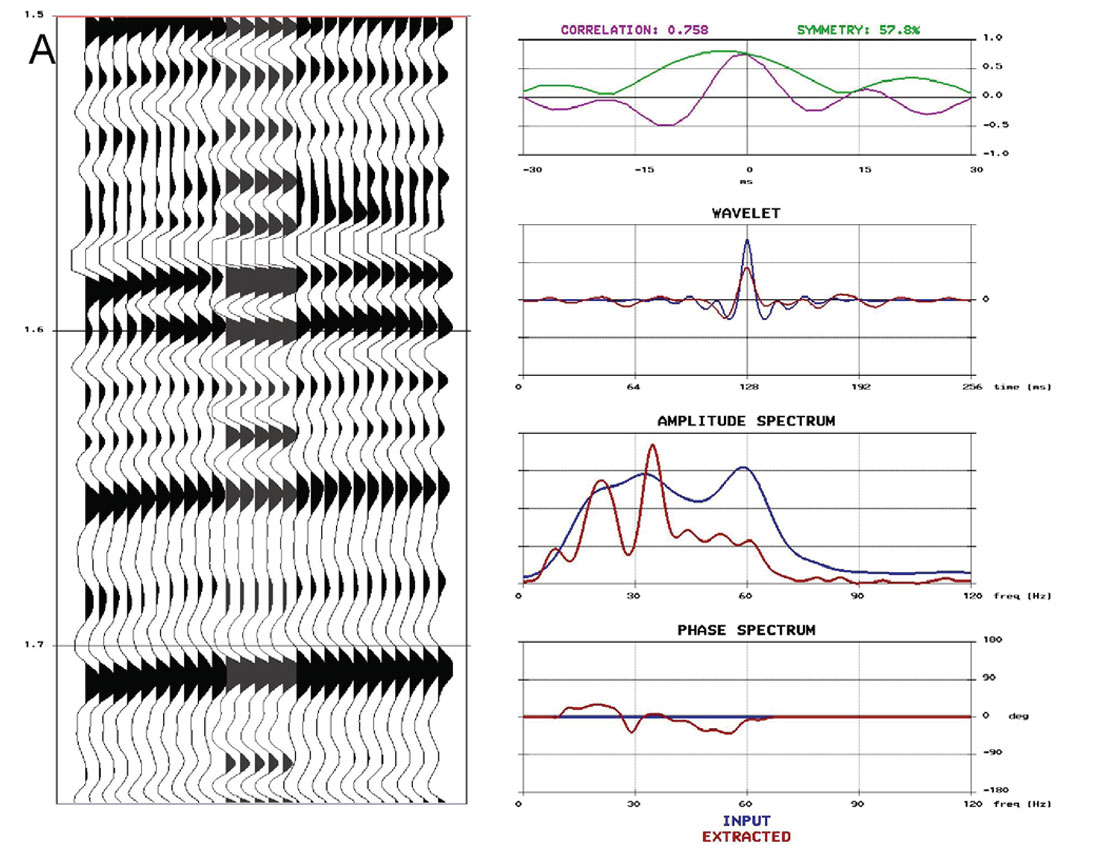
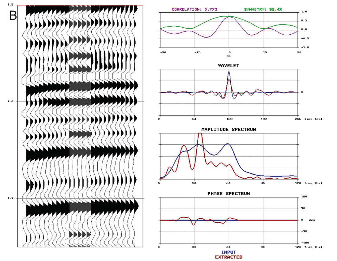
A note of caution when generating comparisons to well logs is that one needs to first assess the quality of the well logs before using them as ground truth. Having multiple wells usually makes this assessment easier, but an in-depth discussion of this evaluation is beyond the scope of this paper. Furthermore, well log tying is not a straightforward process and for a full tutorial on the procedures and caveats, see White and Simm (2003). The discussion here will be based on the assumption that high quality, calibrated well logs are available, and have been correctly tied. For comparisons between stacked data and synthetics, the synthetics are created multiple free with a stationary wavelet that is extracted from a window of the stack centered on the zone of interest in space and time. Figure 1 compares well ties from conventional processing to AVO friendly, well-guided processing. The conventional processing flow in Figure 1A employs a mixture of trace-to-trace and surface consistent processes for deconvolution, ground roll attenuation and scaling. Figure 1B shows the seismic data resulting from careful attention to the amplitudes, using well-guided analysis for parameterization of all surface consistent deconvolution and scaling; surface consistent scaling has been applied after every major stage of deconvolution or noise attenuation. Near-offset stack data is shown here, though the same analysis can be done for the middle and far offsets, as well as for the full offset range. Note there is an increased correlation with the well synthetic in Figure 1B compared to Figure 1A. The ultimate goal is to progressively improve the well tie during processing, so that minimal additional scaling and wavelet shaping is required for inversion.

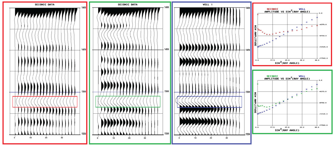
Pre-stack comparisons of the broad AVO trends in the seismic gathers against those predicted by synthetics generated from well logs ensure they match as closely as possible. An example of such a pre-stack AVO comparison is shown in Figure 2. In the well-guided processing flow, signal-preserving ground roll removal was performed iteratively before and after deconvolution, and factored into the surface consistent deconvolution operator design. The clear result is that the AVO curve for a reflector in the zone of interest matches much better during the well-guided processing flow. In the conventional processing flow, the mismatch at near offsets due to noise and ground roll effects is obvious. On the far offsets, the general AVO trend of the seismic gather from the well-guided processing more closely matches that expected from the well synthetic. It should be noted that the offset synthetic shown in Figure 2 was created using offset dependent wavelets.

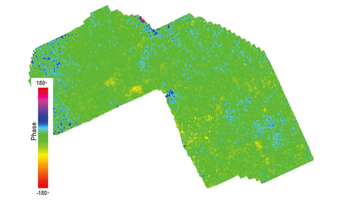
One last comment is that the well-guided processing discussed so far can and should be extended beyond the well locations. One useful tool for this is the examination of horizon based instantaneous attributes, as these can identify anomalies between the wells (Perz, 2004). Figure 3 shows a map of instantaneous phase, extracted along a horizon of interest in a merged 3D seismic volume. This should be done on a full and offset limited stack to verify that no spatial biases are evident, and that the wavelet phase is stable throughout the volume. While there are no biases seen for the example in Figure 3, if the opposite were true, the instantaneous attribute can serve as input data to derive correction operators.

Velocity

A significant aspect of seismic imaging is velocity analysis, whether for complex depth imaging or more straight forward stacking. While depth imaging relies heavily on the geologic accuracy of the velocity model, time migration and stacking processes are usually more forgiving. A common goal is to optimally flatten the gathers and produce the best possible image. Achieving that goal in the case of time imaging, which will be our focus from hereon, can come at the expense of obtaining geologically relevant velocity models. It will be demonstrated that incorporating well information and picked horizons for this purpose greatly improves the quality of the derived interval velocities. In turn, this benefits subsequent time-to-depth conversions, and can serve to constrain the low frequency velocity model used for inversion.

A common approach for picking stacking or root-mean-squared (RMS) velocities is through semblance analysis of common-offset common-mid-point (CMP) gathers at preselected control points. Once picked, they can be interpolated spatially to provide velocity information at each image location. Semblance is a measure of stack power as a function of velocity and time. The velocity associated with a peak in the semblance is chosen as the RMS velocity (V_n ) for the traveltime (t_n). Interval velocities (V_i ) are calculated from these velocity–time pairs using a regular Dix Inversion where

For simplicity, we will keep to the isotropic definition of stacking and interval velocities and refer to Grechka et al. (1999) for an extension to anisotropic media.

There are two main strategies for semblance picking. The first is the quickest to implement and consists of picking large semblance values wherever they exist, regardless of spatial consistency. This requires some form of interpolation in the time direction prior to interpolating the function laterally between control points and deriving interval properties. The second strategy is more elaborate and involves picking the semblances along the main geologic interfaces, particularly at significant interval velocity changes. Ideally the wavelet should approach zero or minimum phase, and spatial variability in phase should be negligible along the picked interfaces so that velocity control points can be placed consistently (see again Figure 3). Picked horizons and well logs are incorporated into the velocity analysis and serve as a guide, ensuring that the calculated interval velocities match the well and track the correct event. Using these guides can also help in difficult data areas where the true velocity changes are obscured by noise, multiples, or strong energy events such as coals. In this second strategy, spatial interpolation between control points is more straightforward, provided that each individual point accurately and consistently describes the geologic velocity function, and that there are sufficient control points to capture spatial variability.

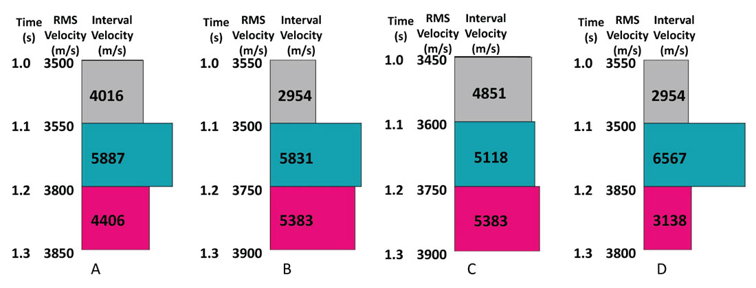
Stacking velocities are very robust and both picking strategies will often yield similar images, particularly in the deeper part of a section. This is not the case for the associated interval velocity fields. To illustrate the benefits of well-guided velocity analysis we first consider a simple synthetic model with four reflectors, as described in Figure 4. Within this model, a 50 m/s (<2%) error in any stacking velocity pick translates to a maximum of 4 ms of moveout error at 2000 m offset (approximately 35-40° incident ray angle at this depth in this model). This picking error is well within the range of what is achievable in typical and reasonably flat geologic settings, with the exception of some very shallow targets. Figures 4B to 4D, as compared to Figure 4A, show that these small stacking velocity changes can result in very large interval velocity differences, in some cases enough to even change the sign of the interval velocity contrast.

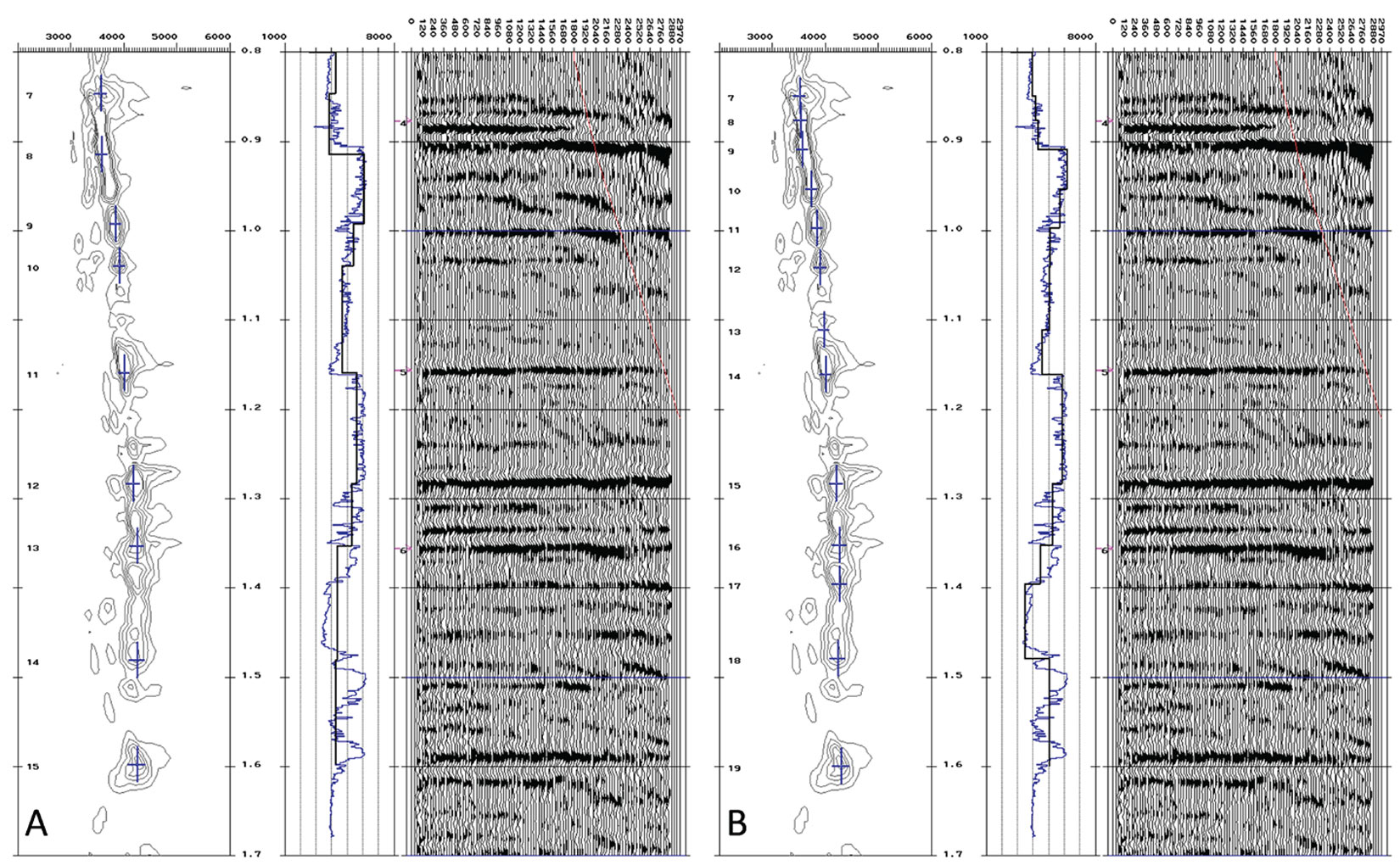
The two velocity analysis panels in Figure 5 show similar results. The velocities for Figure 5A have been picked by targeting the strong semblance clouds, while the velocities for Figure 5B have been picked in a more geologically correct manner, using well information and picking along the major velocity boundaries. Small changes to a picked RMS velocity are applied where necessary to produce the desired interval velocity, without significant change to the NMO corrected gather. Both approaches have worked equally well at flattening the gather, however the well-guided approach has a much better interval velocity match to the well log.

One use of these interval velocities is in depth conversion, where a smooth version of the velocity field is required. If care has been taken in maintaining geologic consistency, the need to use a large spatial smoother may be avoided, and this reduces the risk of smoothing through real variations in the velocity field. Lateral variations in the true velocity field can distort the subsurface structure if not properly accounted for in the depth conversion. The inverse also holds true, as using an unrealistic velocity model for the depth conversion will also result in an erroneous depth structure.

The images in Figure 6 show a dataset from northeast British Columbia. The top three panels show the results using a methodology focused simply on flattening gathers, and the bottom three panels show the results using a geologically constrained velocity analysis approach. The left panels show the time stack and associated RMS velocity field. Notice the similarity of the velocity field and how only very subtle differences are observed in the two stacks. The middle panels show the same stack but instead with interval velocities. Small changes in the picked RMS field have resulted in lateral discontinuities and a non-geologic velocity field on the top middle image. The right panels show the depth converted sections, using the interval velocity field from the middle panels. Significant structural differences attributable to the differences in the velocity field are observed between the two sections. Overall the depth converted section derived from the geologic velocity model (bottom right) better maintains the general structural characteristics of the time section and looks more geologically reasonable.

Inversion

The low frequency model is one of the most important factors in the derivation of rock properties from AVO inversion, because it determines the overall values of the inverted quantities (as opposed to local relative changes). This section will discuss how the velocities obtained from the well-guided workflow described above can be used for the creation of the low frequency model for simultaneous model based AVO inversion. A particularly important factor is the interpolation of the low frequency model between the well locations. Guiding the low frequency model with event times is necessary, but not sufficient. Additional lateral guides are needed when the wells show changes in a quantity within a given layer. Where between those wells should the low frequency model increase or decrease? One way to solve this issue is with co-kriging, where the interpolation of data between the wells is augmented by another variable that guides the results; interval velocity for example (Petrowiki 2017). Interval velocities, when picked geologically as described in the previous section, guided by interpreted horizons and well control, can show a co-kriging algorithm where to implement a given increase, rather than just applying gradual grading.

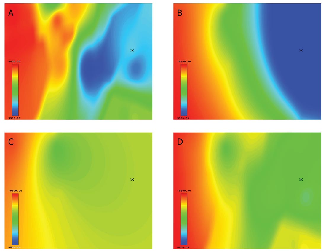
To that end, an experiment was performed using a seismic volume that contained several wells. The wells located towards the west side of the survey were used to generate the low frequency model, and the well on the east side was left as a blind well. This may be a bit extreme of a situation, where the well control is confined to one side of the volume, but it illustrates the point nicely. Figure 7 shows the derived low frequency models extracted along a reflector-guided slice. Figure 7A shows the interval velocities along the reflector-guided slice. There is a trend of decreasing velocity from west to east, and the lowest velocities are found in the region towards the northeast (the blue region in Figure 7A). In Figures 7B and 7C, the result of pure (well-only) kriging of the P-wave impedance on this slice is seen. Figure 7B uses all available wells, and clearly exhibits the west to east trend of decreasing impedances, although with nowhere near the detail of the interval velocities. Figure 7C uses only the wells on the west side of the region. There is no way for the kriging algorithm alone to guess the extent of the decrease of impedance from west to east. Figure 7D shows the co-kriging result, using only the wells in the west, but guided by the interval velocities from Figure 7A. Some of the details of the interval velocity image begin to show up, and the observation is that the low frequency model matches more closely that of Figure 7B. If the only wells available were those in the west, co-kriging using the interval velocities would have definitely produced a more accurate low frequency model of P-wave impedance than kriging alone, but only if one has confidence that the interval velocities are geologically sound.

Further to this, the inversion results were examined at the location of the blind well to the northeast, within the low velocity channel (the “X” in Figure 7). Figure 8 shows P-wave impedance (left column), S-wave impedance (middle column), and VP/VS (right column) for each of the models described in Figure 7B (top row), Figure 7C (middle row), and Figure 7D (bottom row). The top row represents the ideal case, where all available wells were used. In the middle row, we see that the inverted results are systematically too high as compared to the well log profiles for the P-wave impedance and the S-wave impedance (only the P-wave impedance was shown in Figure 7). Since both the P-wave and the S-wave impedances are off by the same percentage, the VP/VS happened to come out about right, but this is a coincidence. In the bottom row, the P-wave and S-wave impedances have been corrected to much lower values, and this has not happened at the expense of the VP/VS ratio. The average percent difference between the inverted result and the well log profiles on the bottom row has been cut to near the ideal case on the top row, for the P-wave impedance and the S-wave impedance, and again, the VP/VS ratio percent difference has not been harmed. In this case, co-kriging using the well-guided interval velocities has given us a result at a blind well that is nearly as good as it would have been had the well been included.

Conclusion

Situations have been shown where a proper well-guided seismic processing workflow produces improved results to conventional seismic processing workflows, for the purposes of both interpretation and pre-stack analysis. Well-guided processing ensures that every processing step improves well ties for both stacks and gathers. Picking the best possible well-guided velocities can seem irrelevant for basic time processing, but its benefits are revealed during time-depth conversion and amplitude inversion. Admittedly, geologically guided velocity analysis does take more processor effort, and often requires close collaboration with interpreters, particularly in complex geologic settings. However it is fair to say that the benefits are worth the extra effort. Well-guided processing with its associated quality control aids interpretative stages beyond stack interpretation, into amplitude inversion and depth conversion.

Acknowledgements

The authors would like to thank Wayne Hovdebo and David McHarg of Progress Energy for the velocity data example and for their contributions to this work. Thank you Pulse Seismic for providing show rights on their seismic data. Thank you to everyone at Earth Signal Processing Ltd. for the processing and preparation of the data examples, and special thanks to Faranak Mahmoudian for useful discussions and feedback on this paper.