Advanced seismic techniques help in characterizing a challenging Jean Marie carbonate play, NE British Columbia, Canada – a Case Study

Introduction

This paper describes a workflow that was adopted for understanding the porosity and permeability distribution in the Jean Marie carbonate play in British Columbia, Canada. It makes use of some advanced seismic techniques and holds promise of being a robust methodology that has resulted in enhanced deliverability and recovery of gas from this unconventional carbonate reservoir.

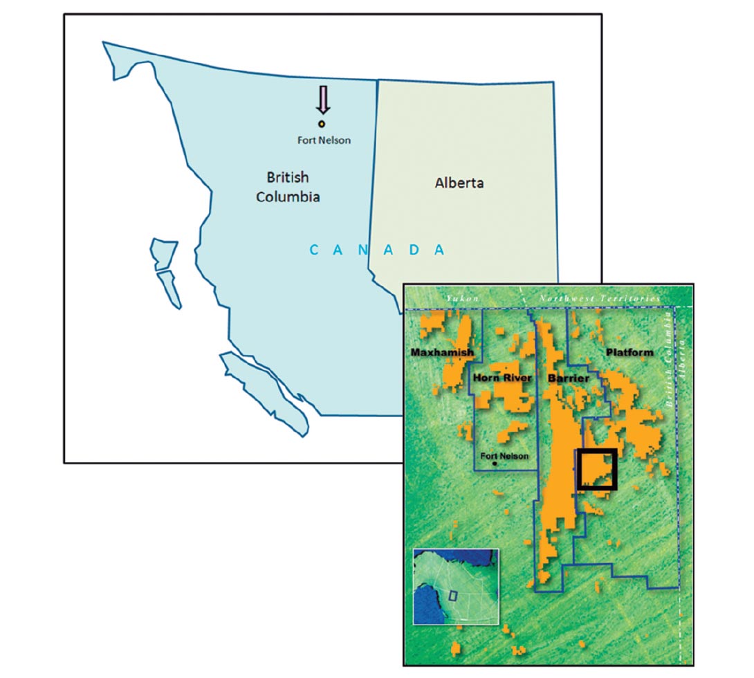
The Jean Marie carbonate platform is located in the Fort Nelson area of northeast British Columbia, Canada (Figure 1). It is a tight, thin and heterogeneous gas bearing carbonate reservoir. The relatively brittle limestone is sandwiched between two ductile shale units – the Redknife and the Fort Simpson shale. In addition, the Jean Marie is draped over the older Keg River and Slave Point carbonate margins and patch high-relief reefs, which lead to additional local fracturing and faulting. Gas is regionally trapped in moderate porosity and low-permeability stromatoporoid-renalcid limestone reef mounds and limestone inter-mound sediments.

The pool is being developed using underbalanced horizontal drilling to obtain commercial gas production from this enormous unconventional reservoir. The "underbalanced" horizontal technique which allows the reservoir to flow the gas back while drilling, results in the quality of the zone being immediately determined. The planning of a horizontal well path as well as impromptu vertical/lateral changes to geosteer the bit to encounter the best anomalies/reservoir relies heavily on seismic interpretation and the guidance it can yield.

The use of advanced seismic techniques to detect porosity zones and high permeability fairways has increased deliverability and recovery of gas from the Jean Marie carbonate. Wells encountering the fracture zones and the associated enhanced porosity and permeability areas in proximity to the open fracture networks have proven to be the best wells with gas rates of over 10 mmcf/d and with consistent gas increase, compared with a conventional well on the average producing 2 – 4 mmcf/d.

EnCana has been developing the Jean Marie unconventional gas field for the last decade. Recent estimates of gas in place are on the order of 283 billion cubic meters (10 trillion cubic feet) and recoverable reserves estimated at 184 billion cubic meters (6.5 trillion cubic feet) (Adams et al 2006).

Geological Overview

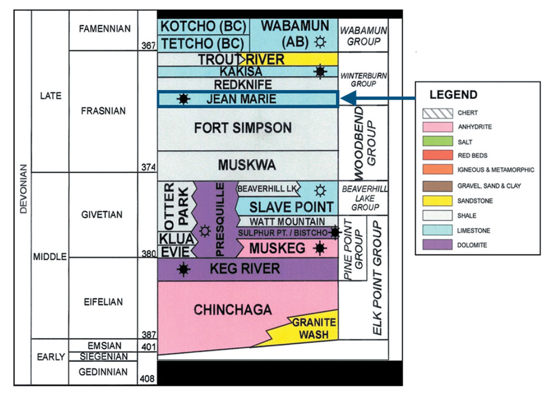
The Jean Marie formation of NE British Columbia is an Upper Devonian (Frasnian) aged carbonate deposited in a ramp type setting on the edge of the North American craton. It is the basal member of the Red Knife Formation (Figure 2) and overlies the shale of the Fort Simpson Formation and is overlain by the thinly bedded shale, silts and limestone of the middle and upper Red Knife formation.

Jean Marie deposition was greatly influenced by antecedent highs of older, deeper Devonian carbonates of the Slave Point and Keg River margin edges and the reefal development along these margins. The deeper Devonian development was in turn controlled by deep seated faults. The subsequent drape and compaction of the Jean Marie over these underlying highs has resulted in fracturing and faulting within the Jean Marie.

In addition to fracturing and faulting associated with the drape over deeper Devonian development, additional fracturing was caused by compression during the Larimide Orogeny, with maximum horizontal stress trending NE-SW or roughly perpendicular to the foothills. This fracture pattern and associated orthogonal sets has resulted in the Jean Marie being heavily fractured and faulted (Hamilton et al, 1995) and, more importantly, with subsequent enhancement of porosity and permeability. The fracture networks appear to have controlled the distribution of hydrothermal fluids which enhance the porosity and permeability of the carbonate via dissolution and recrystalization.

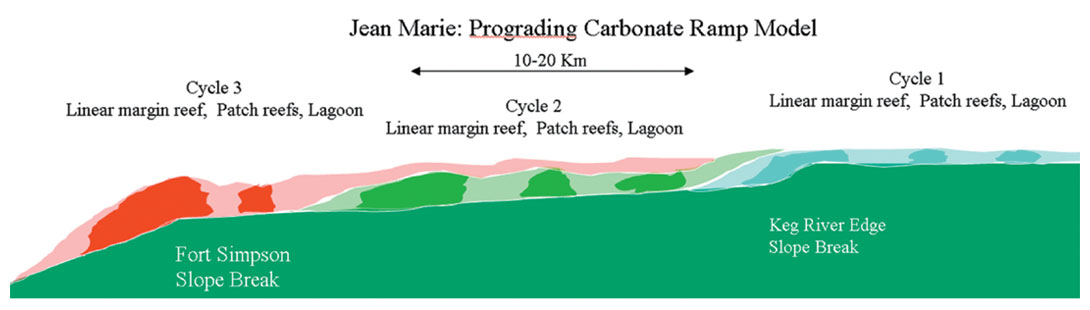
In a regional sense, the Jean Marie thins from west to east and is made up of a series of aggrated, north-south trending reefal margins on the western edge which correspondingly have the thickest development (50 to over 90m). Reefal development within the Jean Marie is predominately by stromatoperoids with minor coralline development. Pendant like encrusting Renalcis, thought to be a cyano like bacteria, grew on and within the stromotoperoid build ups and debris. Westward of the Jean Marie barrier it plunges into the deeper water shale of the Ft. Simpson. Eastward of the reefal barrier the major facies is smaller patch reef development along with associated inter-reefal bioclastic debris shoals and lime mud on the shallower water platform (Wierzbicki et al, 2008)(Figure 3). The Jean Marie on the “platform area” has thicknesses of 20 – 40m and further eastward, towards the Alberta-BC border, thins to 10 – 15m thick. Further east, into present day Alberta, the Jean Marie terminates into thin inter bedded lime mud and shale.

Most primary fabric in the Jean Marie was destroyed during burial with much of the primary porosity plugged by calcite. Subsequent diagenesis by hot brines and fluids moving along fractures and faults resulted in the leaching of some reefal material, but more importantly from a reservoir point of view, bands of encrusting Renalcis. This has resulted in vuggy (avg. 5 – 7%) and micro vuggy porosity (avg. 3 – 6%) within the reefal , Renalcis) and bioclastic shoal facies. In addition, some of the micritic mudstone matrix has been altered to a dolomitic grainstone with micosurcosic fabric and, at times, up to 4 – 6% porosity. Permeability ranges from very tight, with less than 0.5mD, to as much as over 10mD in some cases. The average reservoir parameters are porosity of 4 – 6 % and permeability of 0.5 – 2.0 mD.

Fracture and Porosity Indicators

Fracture detection is an important component in the development of the understanding of this reservoir as these fractures enhance both porosity and permeability resulting in better well deliverability.

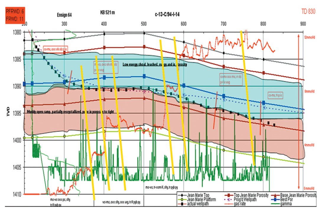
Some of the strongest indicators of open fractures come from the rate-while-drilling (RWD) data obtained while the horizontal wells are drilled (Figure 4). When the wells are being drilled sudden increases in permeability provided by faults or fractures lead to almost instantaneous jumps in gas flow on the order of 1 mmcf/d to 10 mmcf/d. These fracture related permeability RWD changes also show a characteristic rapid drop in rate with time as the fracture is locally depleted. This enables us to differentiate between fracture permeability and permeability associated with high quality reservoir. These major fracture zones may occur every few hundred meters and are generally associated with a seismic discontinuity or lineament.

Detailed description of an origin, controls and interpretation on the nature of the fracture network has been presented elsewhere (Wierzbiki et al, 2010).

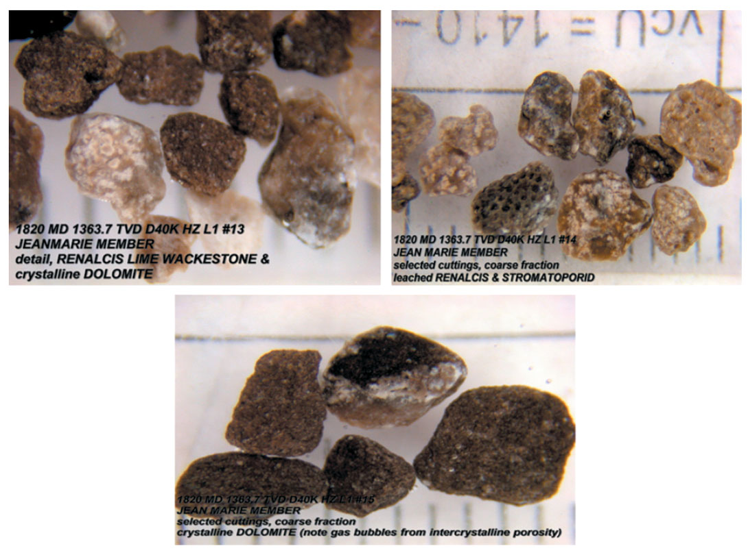
Descriptive indication of porosity comes from good detailed sample descriptions of the reservoir while drilling (Figure 5). The sample descriptions can describe any obvious, direct, porous zones, such as vuggy or micro-vuggy porosity from the reefal or Renalcis facie or intercrystaline porosity of the recrystalized dolomitic facies. However, other more subtle indicators may also be observed and used to interpret where to encounter the better reservoir zones both in a lateral and vertical sense within the Jean Marie. Examples of these secondary indicators are, sample colour, with the reefal facies often being a light cream, beige colour, percentage of secondary calcite, both sparry and massive, which indicates zones of fracturing, leaching and alteration, rate of penetration of the drill bit (ROP), as the better reservoir facies with better porosity drill easier and faster, and lastly, the gamma counts while drilling as the better reservoirs tend to be “cleaner” and therefore have lower gamma counts.

Seismic overview

A 240 sq. km merged 3D seismic reflection data volume was available over the area of interest. Seismic data was provided by Great Plains Exploration.

Historically, prospecting has focused on locating platform interior buildups and linear reef trends which are located on structurally high features. These features have thick isopachs and were assumed to have high porosity throughout the reservoir. For seismic reservoir characterization, isochron, structure and amplitude attributes maps were generated to locate these buildups and design well paths. The variability of permeability and porosity required more advanced seismic attributes to address the issue of reservoir heterogeneity for this thin unconventional reservoir.

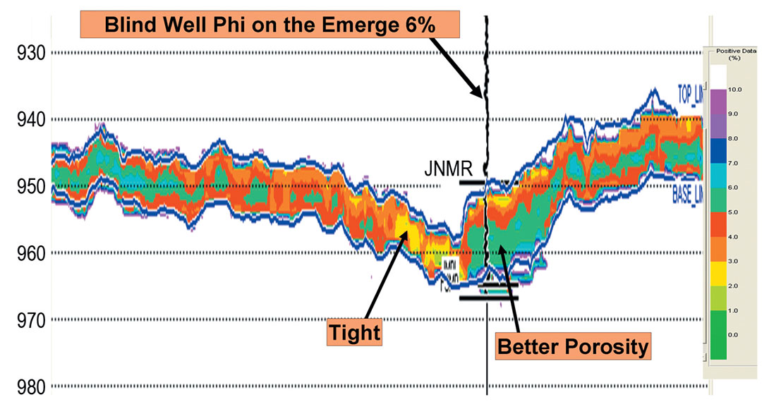
During seismic interpretation/analysis different methods wellsuited for both fracture and porosity determination were adopted. The neural network analysis (Hampson et al, 2001) was used to create 3D volumes of velocity, resistivity, density, neutron porosity, density porosity, effective porosity (Figure 6), Gamma Ray and Vshale. Given the importance of mapping the fracture networks many geometrical attributes were generated such as curvature, dip, gradients, coherence as well as Ant Tracker volume using the swarm intelligence for discontinuity mapping. All above attributes were crossplotted with hard data. The two of them with the best prediction and correlation of known reservoir quality and productivity were neural network predicted effective porosity and swarm intelligence fracture volumes (Figure 7).

The information obtained from integrating these two attributes has been proven to be very powerful tool in identifying the presence of a structure conformable porosity anomaly with the fracture network and drill our best wells to get consistently high gas rate. (Figure 7e).

This study helped to develop a clear enough understanding of permeability pathways and porosity distribution within our reservoir. However, the lack of seismic resolution presented a challenge while drilling, in terms of staying in the best reservoir quality along the full length of the horizontal well (over 1500 m) and not hitting the shale formations above and below. It may be mentioned that the whole reservoir thickness is basically between the Jean Marie peak and the Fort Simpson trough below with net pay thickness varying from 0 – 20m. At the same time the seismic character changes due to reservoir variations (often seen as a doublet in thicker parts of the reservoir) within the platform environment, are very difficult or almost impossible to detect with the use of existing seismic resolution (100 Hz).

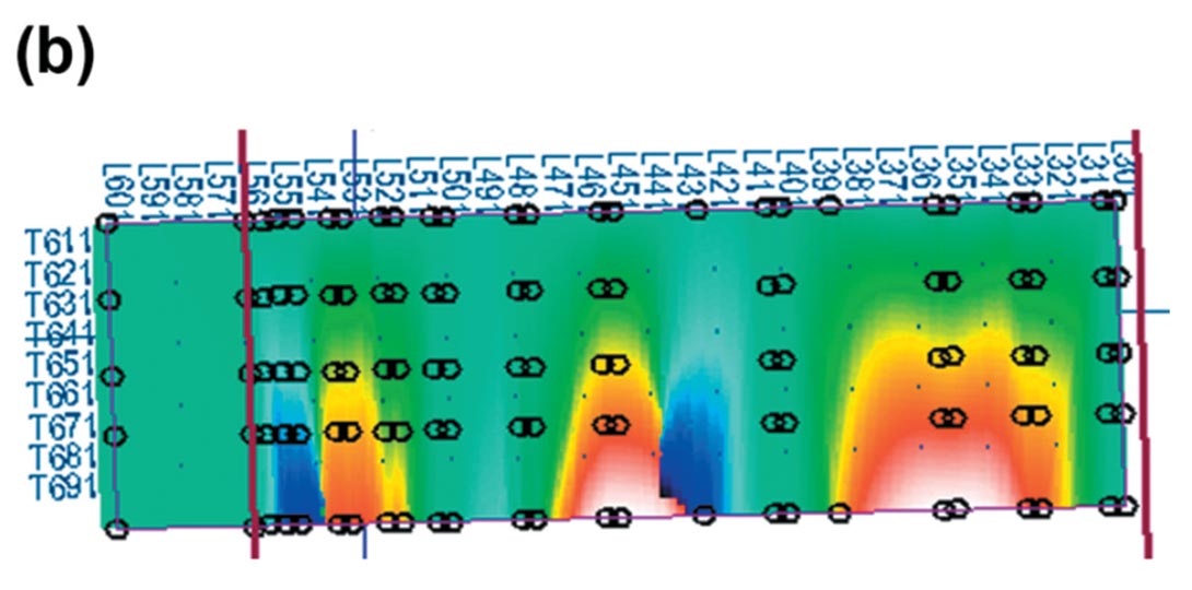
Before embarking on any frequency enhancement process it was decided to determine the minimum bandwidth required to resolve our thin reservoir. For this purpose a complex 3D model was created (Colton, 2008) with variation of porosity as a function of position and thickness.

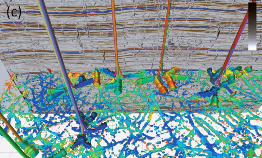
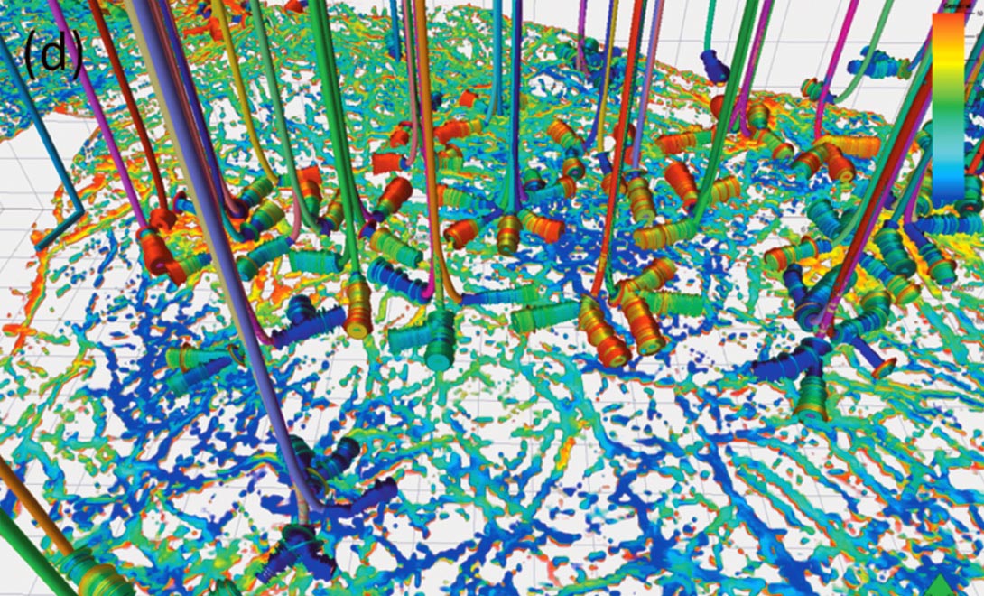
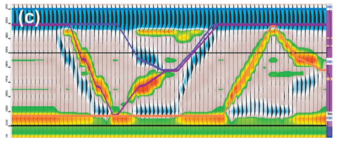
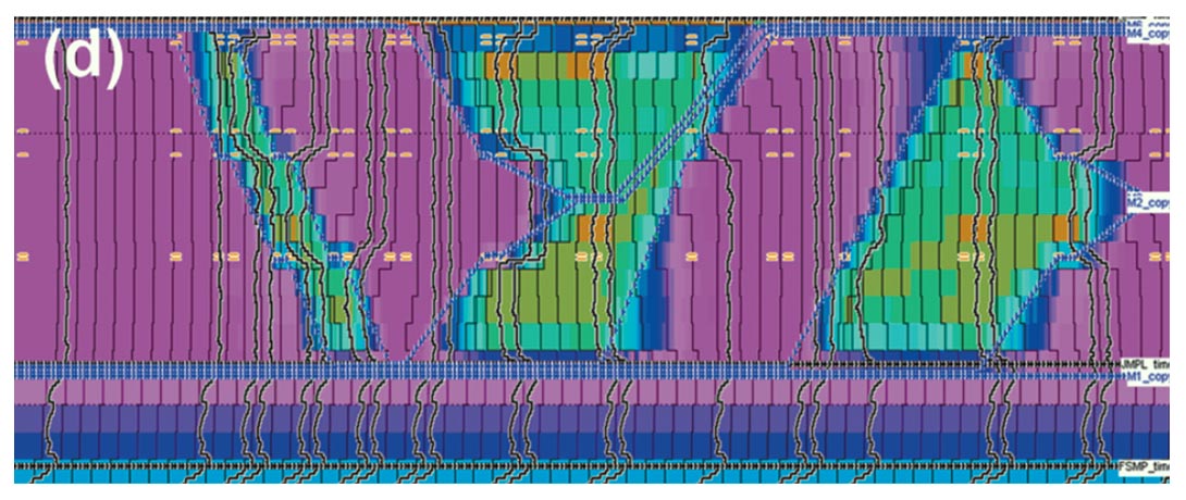
The model consisted of 306 inlines (N-S) and 102 crosslines (E-W), with the same bin size as the seismic (30 x 30m). Logs from 5 wells were used and modified to represent porosity change (% versus position and thickness). Porosity changed along cross lines from the tight 0% (N) to 9% porosity (S), while net pay thickness changed along inlines (Figure 8). As noted, the seismic character changes can be largely attributed to changes in pay quality/porosity and reservoir thickness (Figure 8c and 8d).

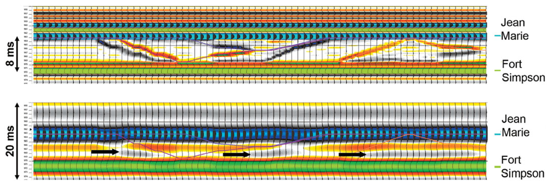
The 3D model demonstrates how the seismic expression changes with both a variable net pay thickness and location (upper, lower, middle) within the Jean Marie – Fort Simpson isopach and investigates the frequency bandwidth required to resolve our reservoir (Figure 9). The modeled reflectivity response was put through a series of filters to determine which frequency bandwidth would be able to detect the seismic character change (from single waveform to doublet), that is indicative of porosity. As shown in Figure 9b, 150 Hz is the frequency requirement for the purpose. To get to that frequency bandwidth, we decided to explore the potential benefits of thin-bed spectral inversion.

Thin-bed reflectivity inversion

Thin-bed spectral inversion is a novel way of removing the wavelet from seismic data and extracting reflectivity (Castagna et al., 2003; Portniaguine and Castagna, 2005; Chopra et al., 2006). It is based on the premise that the spacing between spectral peaks and notches for a windowed portion of a seismic trace is a function of layer thickness in the time domain (Partyka et al., 1999).

In practice, thickness and reflection coefficients can be inverted for as far below the tuning thickness as noise will allow. The 1/8 wavelength Widess limit on resolution only applies if the reflection coefficients are exactly equal and opposite. When there are multiple layers contributing to the seismic waveform and noise, the inversion becomes non-unique, but if we make the reasonable assumption a priori that the reflection response is dominated by only a few layers, one can readily and robustly invert the superposition of sinusoidal layer responses in the frequency domain. The result is an earth model that provides an alternative, and often better, image of the geology than the original seismic trace. If the seismic response results from many fine layers, and/or contains transitional interfaces, or if the seismic data are very noisy, the inverted reflectivity can be sparser than may be desired for interpretation purposes. If the even component of the signal is below the noise level, the resolution achievable falls back to the Widess limit. Our experience has shown that the simple assumption that each seismic reflection is dominated by only a few reflection coefficients, albeit not necessarily the sparsest number, often results in an inverted image that is far superior to the original seismic data for exploration and development purposes.

Puryear and Castagna (2008) described the theory behind the method, and demonstrated its utility by performing layer thickness determination on a real seismic survey without well calibration to achieve estimation accuracies of a few millseconds at time thicknesses approaching 1/16 wavelength. They showed how much more geologically reasonable inverted reflectivity images are from a stratigraphic point of view than are the seismic sections from which they were derived.

As described by Puryear and Castagna (2008), the inversion utilizes spectral decomposition to unravel the complex interference patterns created by thin-bed reflectivity. Spectral shape information as a function of record time, in the form of a timefrequency gather for each original seismic trace, drives an inversion based on the complex superposition of layer spectral responses to obtain the reflectivity. The inverted reflectivity generally has significantly greater vertical resolution than the original seismic data. This inversion process does not require stringent assumptions for its performance. It does not require any a priori or starting earth model, nor any reflectivity spectrum assumptions beyond that implied by the assumption that the earth model is blocky, nor horizon constraints. Neither is a well constraint mandatory, though having one well control point can be helpful for wavelet extraction. For data with high signal-tonoise ratio (SNR), thicknesses far below tuning can sometimes be resolved. Appreciable noise in the data deteriorates the performance of the inversion outside the frequency band of the original seismic data, but the method still enhances high frequencies within the band without blowing up noise as conventional deconvolution would do. This occurs because rather than shaping the amplitude spectrum by spectral division, or its equivalent, which must blow up the noise at frequencies where there is weak signal, the reflectivity output from the inversion process is constrained to a large extent by those spectral bands in the original data where the signal-to-noise ratio is high, and thus noise is attenuated at frequencies where the signal was originally weak.

The output of the inversion process can be viewed as spectrally broadened seismic data, retrieved in the form of broadband reflectivity data that can be filtered back to any bandwidth that filter panel tests indicate adds useful information for interpretation purposes.

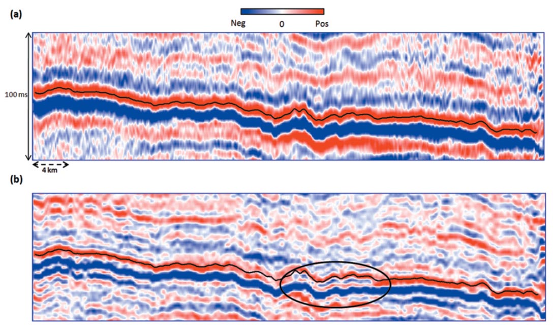
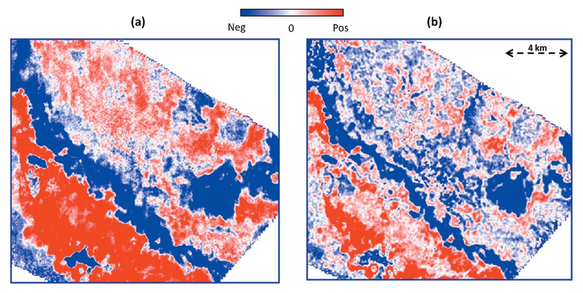
Figure 10 shows a comparison of a segment of a seismic section from the 3D seismic volume under study and its equivalent filtered reflectivity section. Keeping in mind the quality of the input seismic data, the thin-bed reflectivity section looks much better in terms of the noise level as well as extra reflection detail. Based on our modeling study, the reflectivity was filtered back to 150 Hz at the high end, compared to 100 Hz which was the high end frequency of the input data. Figure 11 shows a comparison of time slices from the input data and the filtered thin-bed reflectivity volumes. Notice that blue and red blobs in the input shown in Figure 11a are seen in more detailed reflection patterns in Figure 11b. Thus such a frequency enhanced version of the input seismic allows easy interpretation of subtle stratigraphic features, as illustrated here.

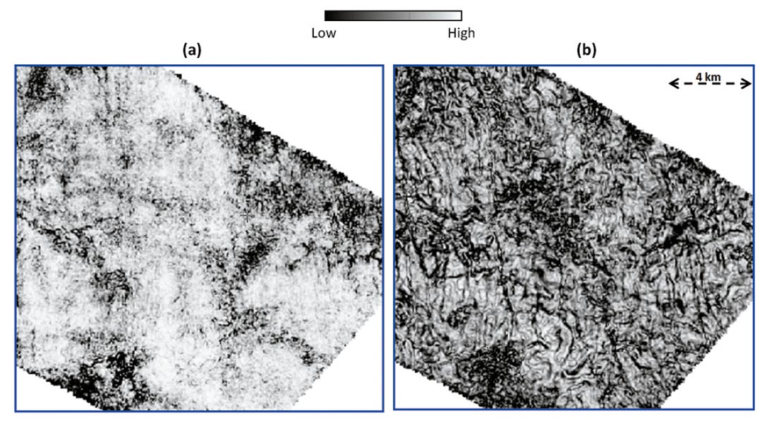
Attributes run on frequency enhanced seismic data yield more accurate results and so allow more meaningful interpretation (Chopra and Marfurt, 2008). Whether it is the mapping of channels, faults/fractures, or subtle onlaps and offlaps, such an exercise always proves useful. Figure 12 shows a comparison of coherence horizon slices in the seismic volume at hand. Notice, the horizon slice to the left does not show any meaningful lineament detail that could be interpreted as faults or fractures. By comparison, Figure 12b shows many lineaments that could be picked up for a more detailed interpretation and confirmation.

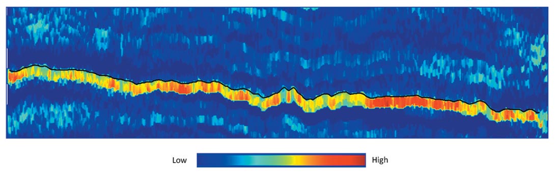
Impedance profiles can be represented as either absolute impedances, which have magnitudes equivalent to the magnitudes of log data measured across targeted intervals, or as relative impedances, which have arbitrary amplitudes that show depth dependent variations equivalent to those exhibited by log data. We emphasize here the advantage of calculating relative impedances from thin-bed reflectivity data (Chopra et al, 2009). When interpreting relative impedance profiles, the top and bottom reflection boundaries of a unit are not correlated with well log curves. Instead, the thicknesses of relative impedance layers are correlated with log curve shapes. Figure 13 shows a sample profile from the relative acoustic impedance volume run on the thin-bed reflectivity volume. Notice the relative variation in the impedance which is not seen on either the input seismic data or just the filtered reflectivity data (also see Figure 16b).

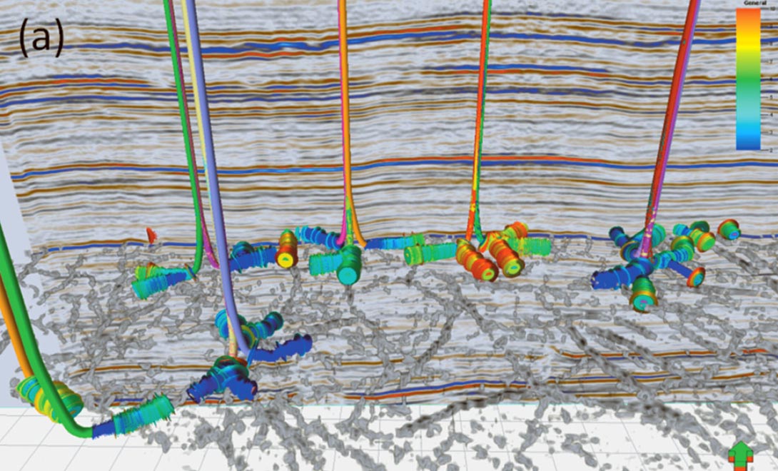
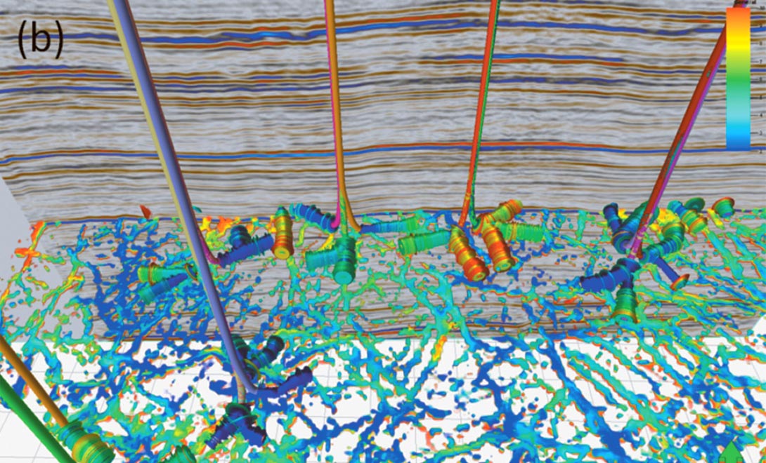
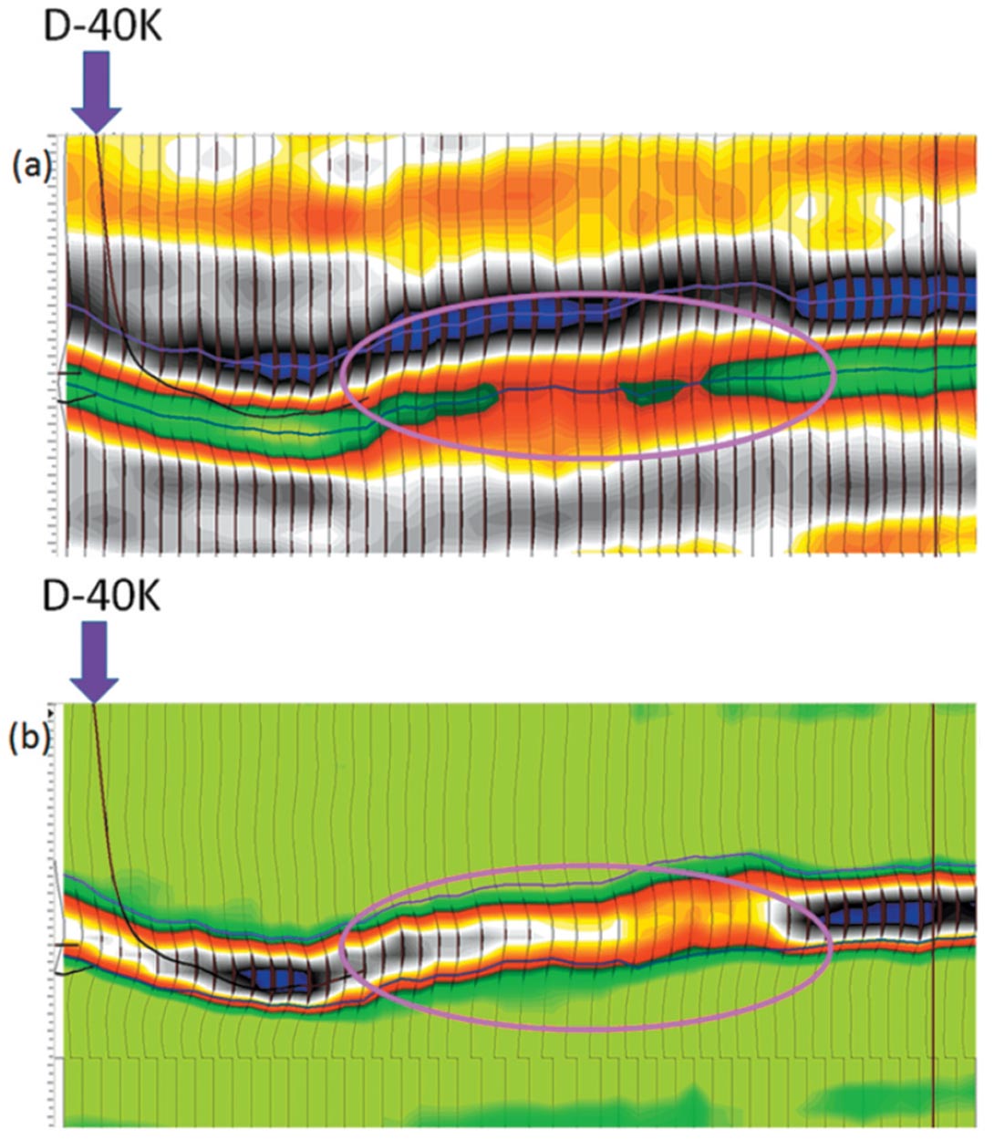
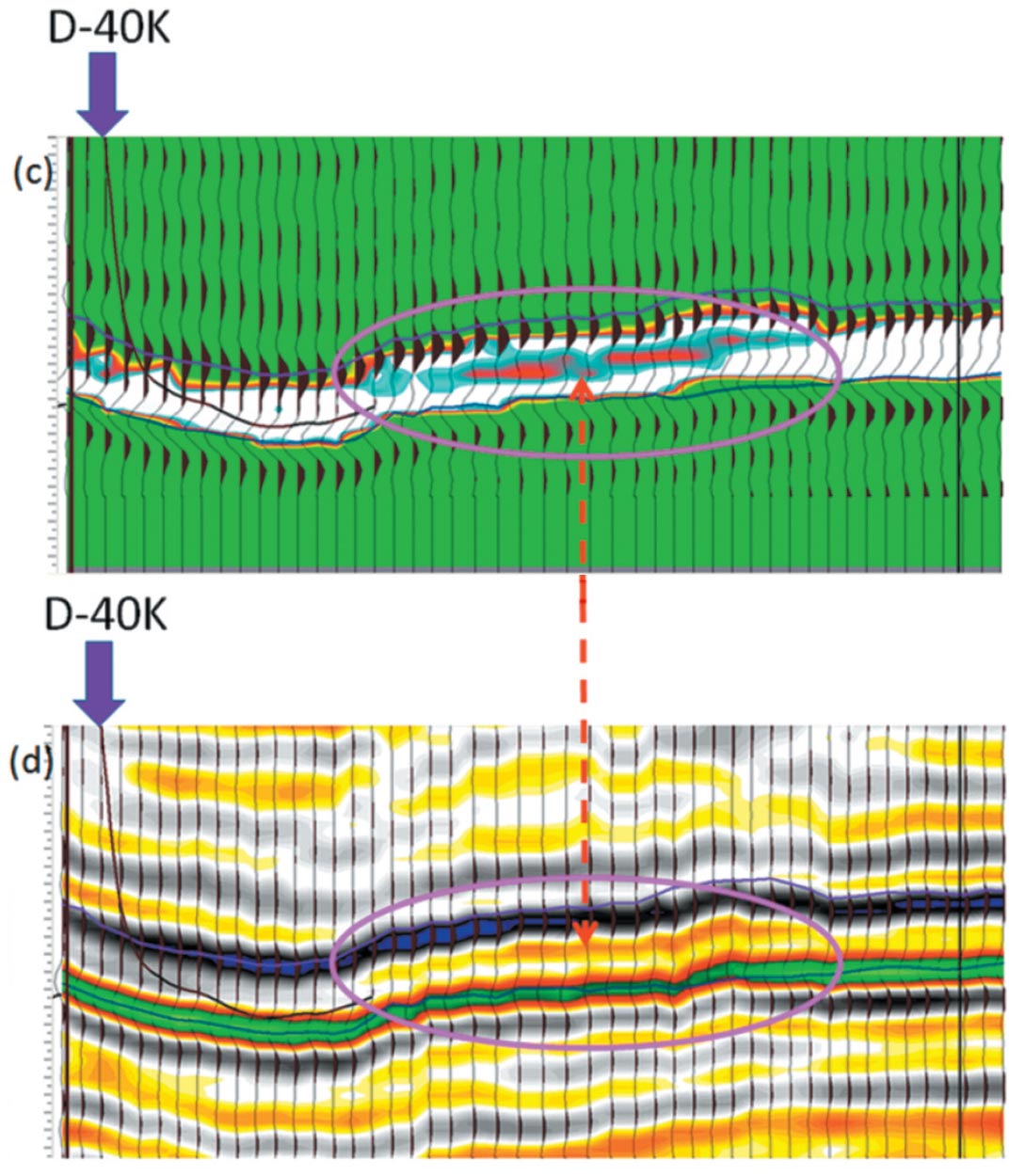
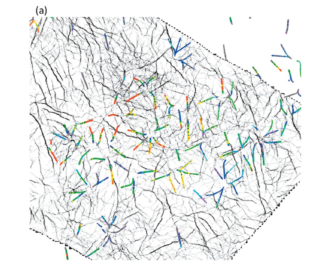
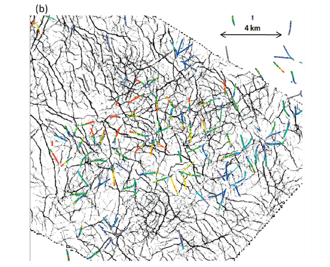
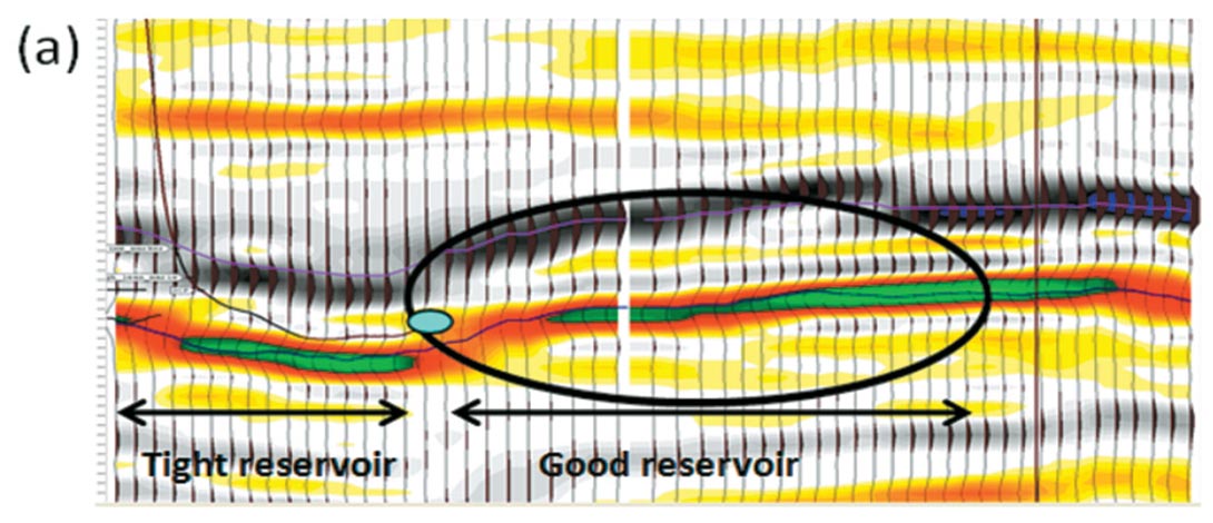
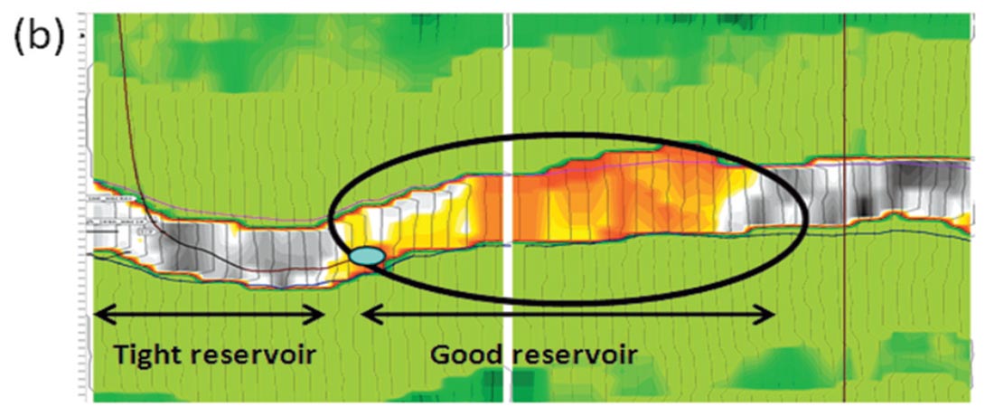
To illustrate the advantages of thin-bed reflectivity inversion and the relative accuracy in interpretation that come of it, we show comparison of profiles from the input seismic data (Figure 14a) and the filtered thin-bed reflectivity (Figure 14d), as well as the acoustic impedance run on the input data (Figure 14b) and the probabilistic neural network effective porosity run on the input seismic data (Figure 14c). Notice the correlation of high effective porosity (in red) seen in Figure 14c with a doublet seismic character in Figure 14d. The reservoir zone indicated with the highlighted circles can be seen clearly. Figure 15 shows a comparison of the Jean Marie horizon slices from Ant Tracker run on input seismic data (Figuire 15a), and Ant Tracker run on filtered thin-bed reflectivity derived from input seismic data (Figure 15b). Overlaid on the fracture lineaments detected by the Ant Tracker are the ribbons showing RWD data from horizontal wells, blue being (0 mmcf/d) to red (10 mmcf/d). We observe a higher correlation of apparent gas kicks when crossing the fractures.

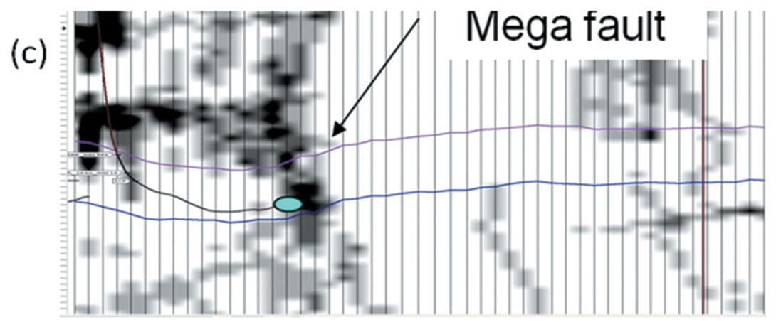
Overlaying fractures and porosity can help evaluate the possible presence of a structure-conformable porosity anomaly on the target horizon connected with the fracture network. Such wells that encounter good porosity in the vicinity of permeable fracture networks generally have the best deliverability and greater associated reserves. This is the recipe for the best wells that one may want to drill. Figure 16 shows a segment of a seismic section from the thin-bed reflectivity volume derived from the input seismic data and along the length of the horizontal well D-40-K. Notice the reef development in the highlighted zone. An equivalent profile from the relative acoustic impedance derived from the thin-bed reflectivity volume is shown in Figure 16b. Notice the lower impedance associated with higher porosity seen in the highlighted zone corresponding to the reef. An Ant Tracker was run on the thin-bed reflectivity volume and an equivalent section to both (a) and (b) is shown in Figure 16(c). The horizontal well which hits the fracture lineament at the blue circle encountered high gas flow rates at that point (details are given in the next section).

Drilling results

An example of one of the exceptional wells drilled in this area this year is the horizontal well D-40-K. Three horizontal legs were planned to target various fractures and the associated altered and enhanced reservoir rock in the immediate vicinity of these fractures, which were identified by thin-bed reflectivity and Ant Tracker seismic volumes. However, due to extremely high gas flow rates and associated pressure encountered from a fracture zone, only 428 meters of the first leg was actually drilled (Figure 17).

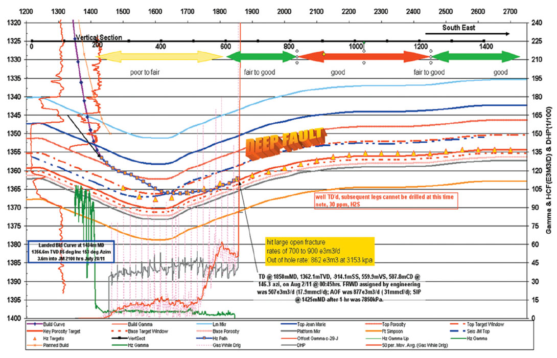
The first horizontal leg drilled out in a microcrystalline, slightly dolomitic wackestone with trace poor porosity (1-2%) and no significant gas flow (as shown to the left of Figure 16a and b). As the first fracture target was approached there was an increase in the percentage of dolomitic packstone and grainstone with a slight increase in porosity and permeability seen in samples (2- 3% porosity, est. 0.2-0.5 mD perm). Gas flows started to increase up to 60 E3M3/d (~2 mmcf/d) while down hole pressures (DHP) were a “normal” 4500 kPa (Figure 17). At 390 meters from the casing shoe a wide fracture zone was encountered (1824- 1831m MD) and gas flow immediately increased to as much as 900 E3M3/D (~25 mmcf/d) with a maximum DHP of 9170 kPa. At this point drilling could not be continued and the well was readied for production and the other two horizontal legs planned from this surface location were dropped.

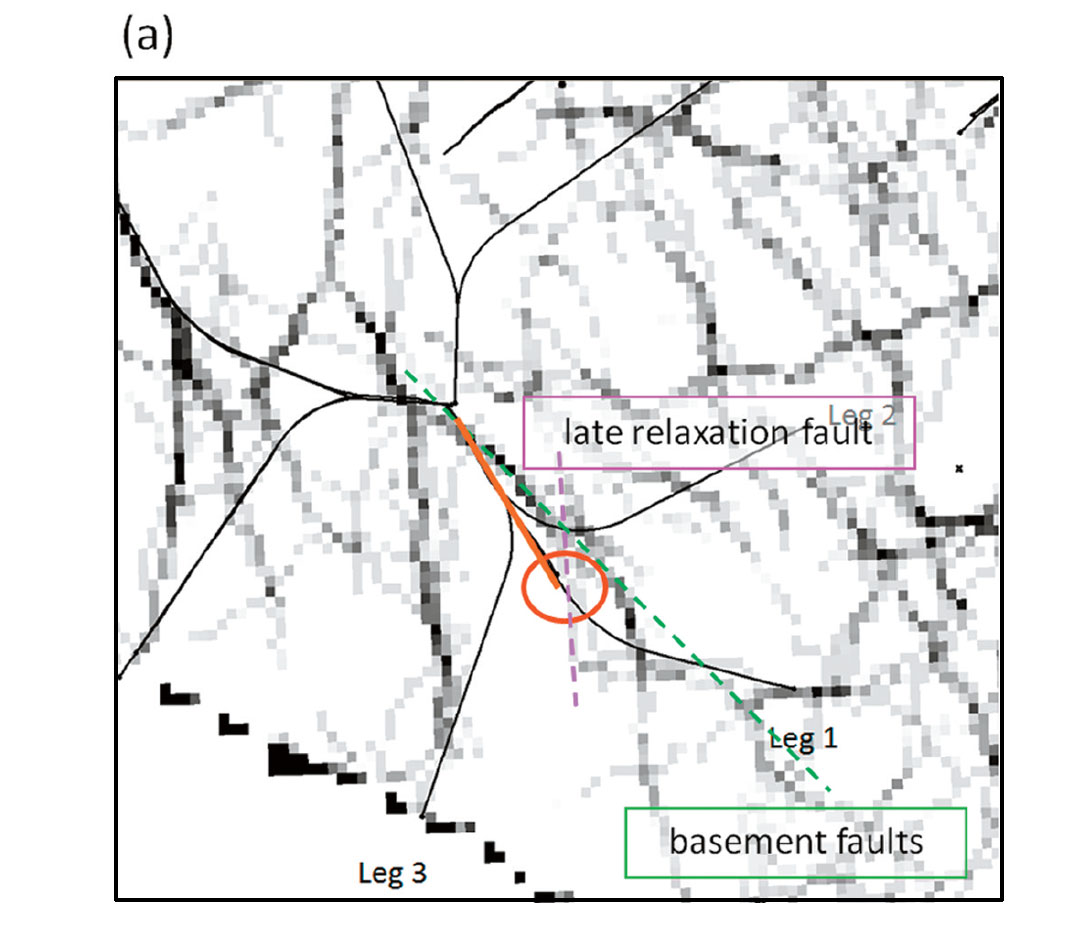
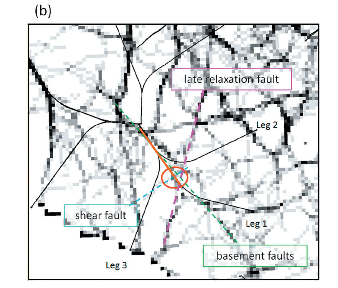
This prompted a review of the seismic data and the derived attributes so as to understand the fracture mechanism at the reservoir level that gave significantly high gas flow rates. Based on our current understanding (Wierzbicki et al, 2010), there are three different sets of fractures in play: North-South oriented relaxation related closed fractures not contributing to productivity, NNE-SSW oriented basement structure and drape related fractures, which quite often are open and so contribute to well productivity, and the conjugate shear related fractures oriented NE-SW, which are often open and are a major contributors to enhanced permeability.

Such fractures are seen on the Ant Tracker volumes. Figure 18 shows horizon slices from the Ant Tracker volumes run on the input seismic data (left) as well as the filtered thin-bed reflectivity (right) volumes. We notice that the basement faults indicated in green on the displays are not seen on the left, but are clearly seen on the right. Similarly, the late relaxation faults are seen clearly on the display to the right, though they do not contribute to productivity. Most importantly, the shear-related fractures are only seen on the display to the right, and these are probably the major contributors to productivity.

Conclusions and Discussion

Since 2008, over 100 wells have been drilled in the study area, and the best wells are the ones that have encountered significant permeability enhancements associated with open fractures and leached carbonates.

The adoption of the thin-bed reflectivity followed by generation of relative acoustic impedance as well as the use of Ant Tracking on frequency-enhanced seismic led to the identification of good quality reservoir as well as the ‘weaker’ reservoir zones. The increase observed in final RWD has also been a solid indicator which confirms that the adoption of the above mentioned workflow has significantly increased our chances of success in the challenging Jean Marie play. Simply put, it helped us, define the highly variable reservoir trends, pick the optimal horizontal well path, identify zones where the reservoir would thin out while the wells were being drilled, and more efficiently plan the drainage, thereby enhancing our overall success. This translated into significant economic benefits in terms of access to higher permeability areas, larger drainage areas, higher production flow rates, slower decline and larger reserves. We expect to make use of this workflow in other similar areas.

Acknowledgements

We wish to thank EnCana and Arcis Corporation, Calgary for the necessary support and encouragement to carry out the work discussed in this paper as well as the permission to publish it. We are grateful to Great Plains Exploration for permission to show the seismic data.

Thin-bed reflectivity method mentioned in this paper is commercially referred to as ThinManTM, a trademark now owned by SIGMA3, Houston. Ant tracker is commercially referred as The Ant Tracker AlgorithmTM, a trade mark of Schlumberger.

Last but not least, we would like to thank Laura Trimbitasu (Schlumberger), Bogdan Batlai (Hampson-Russell) and Penny Colton (now Sensor) for all their help with this project. It is hugely appreciated.