Airborne electromagnetic methods: applications to minerals, water and hydrocarbon exploration

Summary

Electromagnetic methods have a transmitter that carries a current that varies in magnitude as a function of time. This current has an associated (primary) magnetic field that has a similar time dependence. According to Faraday’s law of induction, this time varying field induces currents in conductive features in the ground. These currents have an associated (secondary) magnetic field that can be detected by an electromagnetic receiver. There is no need for the transmitter or the receiver to touch the ground, so electromagnetic systems can be mounted on aircraft and used to cover large areas quickly and efficiently.

In time domain EM systems, the time variation of the current is a switch on, followed by a rapid switch off. In general, good conductors have secondary field responses which decay slowly after the switch off. One example from the Shea Creek area of the Athabasca Basin (northern Saskatchewan) shows that these good conductors can be detected at depths as great as 700m when the conductor is large and the intervening material is highly resistive. Poor conductors have responses that decay away rapidly. The alteration above the Millennium deposit (also in the Athabasca Basin) is an example of a response that decays away in about 300 microseconds. Historically, airborne electromagnetic methods have been most successful for massive sulphide exploration.

Electromagnetic methods are being utilized in the search for fresh water. In an example from Denmark, the method has been used to successfully map the thickness of a freshwater aquifer. Using airborne methods, an area of more than 100 km2 was covered in a few days surveying, where it would have taken months to cover the same area using ground methods.

In sedimentary basins, the decay of the electromagnetic response can be used to infer the conductivity as a function of depth. The shallower part of the section is inferred from the early time data and the late time data is used to estimate the deeper parts of the section. When the ground is about 10 Ohm•m, airborne electromagnetic systems can only see about 300 m deep. Hence they cannot see most hydrocarbon deposits. However, electromagnetic methods have been a useful compliment to high resolution seismic in the search for shallow gas in some of the paleochannels in Alberta. They have also been used to better understand the oil sands environment.

Introduction

Controlled source airborne electromagnetic (AEM) systems were developed after the Second World War to explore for mineral deposits (Fountain, 1998). Electromagnetic systems primarily respond to the conductivity (or the resistivity) of material in the earth. Their primary success has been for discovering highly conductive massive sulphide bodies located in resistive terrain such as the Canadian and Fennoscandinavian shields. Recent improvements in digital acquisition systems, calibration procedures and data processing methods mean that the systems can be used to map stratigraphic features — both near the surface and at depths down to a few hundred metres. This means that airborne electromagnetic methods have also been used with some success in mapping features that can be used to assist in the search for groundwater and for hydrocarbons.

Mineral Exploration Examples

A good example of a mineral deposit discovered with the GEOTEM airborne electromagnetic system is the Storliden deposit. Figure 1 shows the discovery profile collected over the deposit.

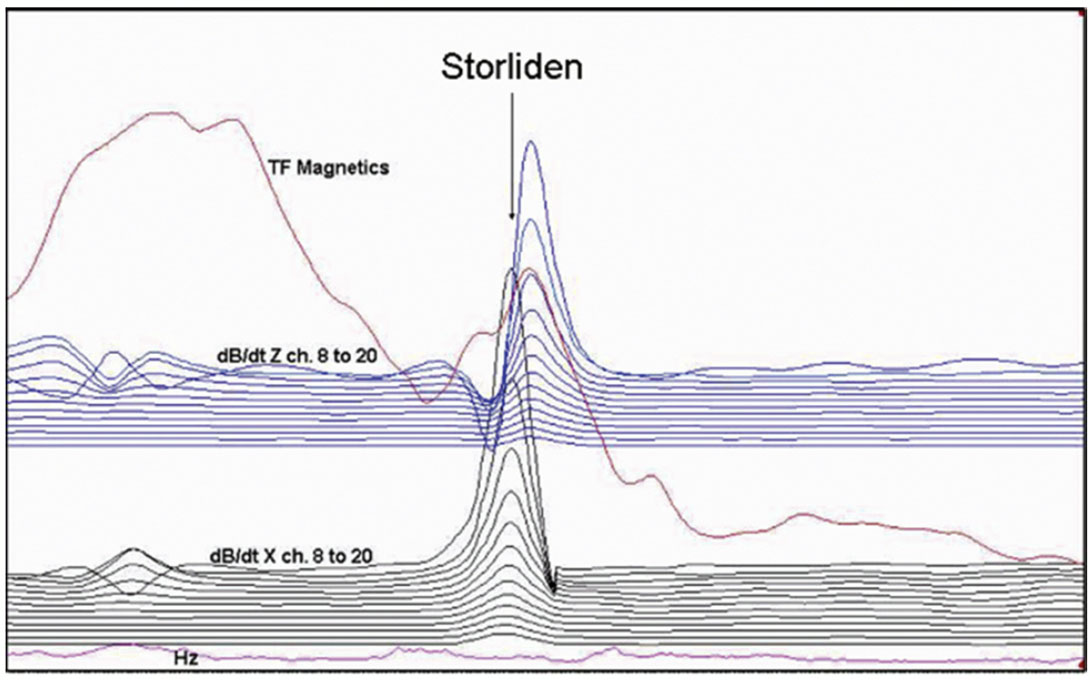
After the anomalous response was judged to be of interest, ground EM (a loop-loop frequency domain system) was used to interpret that the source of the anomaly was a vertical plate-like body. A drill-hole designed to hit this target did not intersect material that would explain the anomaly so deeper penetrating time-domain electromagnetic (TEM) methods were used. The interpreted source of the TEM anomaly was a deeper flat-lying plate. A drill designed to intersect this body hit ore grade material. Interestingly, an interpretation of the original GEOTEM data (Peter Wolfgram, private communication) also suggested a flaylying plate as a source.

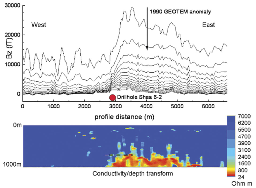
Another GEOTEM AEM survey flown in 1990 over the Shea Creek area in Saskatchewan Canada identified an anomalous response. A large-loop ground TEM survey at the same location was used to identify a conductor interpreted at approximately 800 m depth. A drill designed to test this interpretation struck a conductive zone at 695 m depth. A newly developed high-power AEM system called MEGATEM was able to identify a response associated with this target on a recent survey (Smith and Koch, 2006). Figure 2, shows the MEGATEM AEM profile, with the slowest decay over the deep conductor. In other parts of Saskatchewan, explorers are looking for much more rapid decays associated with more weekly conductive alteration zones that are located above the uranium mineralization.

Water Exploration Examples

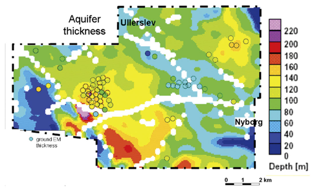
In an example from the Fyn Area in Denmark, the thickness of a resistive aquifer above a saline aquifer was of interest (Smith et al., 2004). An airborne survey was flown to map the depth to the top of the saline layer, which was essentially the thickness of the aquifer. Layered earth inversion (Chen and Raiche, 1998) was used to estimate the thickness from the airborne data. A map of the aquifer thickness for the whole survey area is shown on Figure 3. The colours depict the thickness estimated from ground TEM readings at the location of the circles, while the colours inside the small circles depict the thickness estimated from the ground TEM data. The thicker zones are the ones storing the most water. The agreement between the airborne and the ground data is very good, except in the low resistivity zone on the western edge. Here there are some conductive clays near to the surface that violate our assumptions of a resistor over a conductor, so the thicknesses estimated will not be reliable.

Hydrocarbon Exploration Examples

Mapping gas paleochannels

In recent years, a number of surveys have been flown to map shallow, electrically resistive, paleochannels. These channels can be low-pressure gas reservoirs, but have a very high permeability that means they can be exploited very quickly and economically. In some cases, the sands can be overpressured, creating a hazard when drilling for deeper targets. Hence knowledge of the location and depth of these channels may also be useful for hazard avoidance.

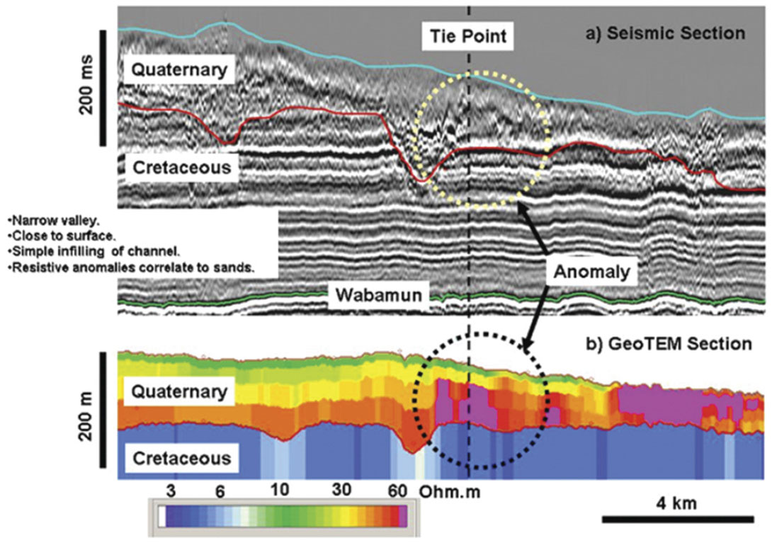
Kellett (2007) has published a case history that discusses four distinct facies of glacial channels incised into Cretaceous sediments and buried below till. One example of a geophysical facies (a narrow valley) is shown in Figure 4. In this case, the Cretaceous Quaternary boundary (red line) shows a number of narrow incised valleys. Within the narrow channel there are some wellbedded strata evident on the seismic section. The location to the right of the central channel is anomalous: It appears as a seismically transparent zone, with no strong reflections on the seismic section. On the airborne EM (GEOTEM) section, the same zone is resistive. Kellett (2007) postulates that these anomalies might be reworked sands in a braided channel system that was subsequently abandoned when the nearby incised valley developed. Note on the resistivity section that the resistivity decreases towards the surface, perhaps indicating a higher clay content that would provide a seal for the gas. Collecting seismic data in this environment requires data to be collected with high-frequency information (up to 70 Hz), small group spacing (<30m) and sufficiently small minimum offsets (<60 m) and large maximum offsets (>1000 m) to get high fold coverage. Also, in the processing, careful attention must be paid to static corrections and nearsurface velocity analysis (Kellett, 2007). The electromagnetic data provides a useful and economical complement to the seismic that can assist in understanding the geological environment.

Mapping Oil sands

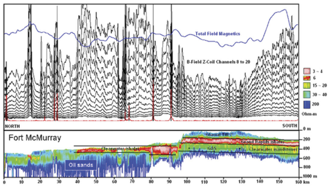
Airborne electromagnetics has also been applied to mapping the bituminous sands in northern Alberta. This data can be used in exploration for oil sands or to provide important information for environmental due diligence and engineering reports. Figure 5 shows a 160 km long profile line flown south from Fort McMurray.

Airborne EM is moderately successful at identifying the more resistive bitumen rich zones where the sands are close to the surface, for example on the left of the section. In other places, where the sands are deeper and covered by the conductive Clearwater shale, it is more difficult to map subtle changes in the resistivity caused by variations in bitumen quantity or quality. However, some interesting research work has been done to show that this might be possible in some circumstances. Although AEM is not always a good tool for direct detection, it could be useful in other circumstances. For example, identifying where the groundwater in the sands are saline or fresh. Another use of the airborne EM data is mapping the continuity of the seal above the reservoir; this information can be useful for planning in-situ recovery.

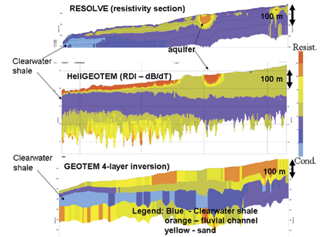
A good example of data collected in an area north of Fort McMurray, Alberta, is shown on Figure 6. The area has Pleistocene sands at surface, overlying the conductive Clearwater formation, which in turn overlies the bituminous McMurray formation. The helicopter frequency-domain airborne RESOLVE system has the best spatial resolution and the highest frequencies, so it has identified a resistive aquifer (labeled orange feature) near to the surface on the resistivity section. It has also identified the more conductive (purple) Clearwater formation below this, but does not penetrate more than 50 m on the left and 150 m on the right. The helicopter time-domain HeliGEOTEM data presented as a resistivity section shows the aquifer and the Clearwater as a horizontal layer (with sands above). There is also an indication of the more resistive McMurray formation below. In this environment the depth penetration of HeliGEOTEM is more than 200 m. The fixed-wing GEOTEM section is presented as a four layer inversion. Again, the Clearwater shows as a horizontal conductive feature. There is an indication of the resistive McMurray further to the right (implying the depth penetration is good), but no indication of the aquifer near-surface (implying the resolution of the fixed-wing systems is less).

Conclusions

Airborne electromagnetic methods can be a useful tool to assist in the exploration for minerals, groundwater and hydrocarbons. For mineral exploration AEM is an established tool.

The use of AEM for groundwater exploration is increasing as it is providing valuable information. The greatest success has been in identifying the depth to saline layers and in some cases the thickness of these layers. Resistive zones might also be indicative of greater porosity or fresh water and these are most evident when not covered by conductive layers (clay or saline water).

The depth penetration of a few hundred metres is very limiting in the direct detection of hydrocarbons. Airborne EM can be useful for identifying paleochannels, which in some cases might contain gas. The gas could be a drilling hazard, or alternatively, could in some cases be exploited economically. In some cases AEM could map facies variations within the paleochannel that might be associated with a gas reservoir.

In the oil sands, airborne EM can be very useful when the sands are not covered by conductive shales. In this case, high resistivity can correlate with more bituminous material. In cases where the sands are covered, the AEM data can be used for determining the quality of the seal and planning in-situ recovery. These latter factors do not impact on exploration, but on production.

Acknowledgements

I would like to thank Richard Kellett for feedback on the use of AEM to map paleochannels. The Storliden data is shown courtesy of North Atlantic Natural Resources AB. This work was completed while I was working with Fugro Airborne Surveys. I am grateful for their support.