Analyzing a Seismic Pitfall – Pliocene Superdeep High Amplitude Anomaly, Offshore, Bay of Bengal, India

A wildcat was drilled on a Pliocene superdeep seismic high amplitude anomaly in 1050 m of water to explore the hydrocarbon potential in the bathyal zone of Bay of Bengal. The well penetrated a thick monotonous section of 1400 m of siliciclastic mudrocks without encountering the prognosticated hydrocarbon sands, resulting in a seismic pitfall. Post-drill analysis shows intriguing inconsistencies between the rock properties and their seismic response; high amplitude reflections are seen without matching impedance log contrasts, while strong contrasts in logs do not show corresponding amplitudes in seismic. Prestack elastic gather modeling indicates the high amplitudes seen in normal stacks could have been caused by large VP /VS contrasts within the mudrocks, without having the requisite P-impedance contrasts. However, the reasons for poor seismic reflections against appreciable contrasts in logs are not quite clear.

Introduction

The southern part of the Indian east coast offshore, the Krishna-Godavari and Cauvery basins in the Bay of Bengal are long known oil and gas provenances in both shallow and deep waters. But the offshore Mahanadi Basin to the north so far has eluded success though a number of wells are drilled in shallow and deep waters nearer to the coast. Much further to the east in the unexplored bathyal zone of the Bay of Bengal, a wildcat was proposed and drilled in 1050 m of water on a Pliocene high amplitude seismic anomaly of sizable area, to explore hydrocarbon potential in this part. The well, however, penetrated 1400 m of hemipelagic siliciclastic mudrocks without encountering any of the prognosticated hydrocarbon sands and resulted in a seismic pitfall which required investigation. Seismic calibration with well revealed intriguing discordances between the impedance contrasts recorded in logs and their amplitude response in seismic prestack time and depth migrated (PSTM and PSDM) data. This led to the inaccurate interpretation resulting in the pitfall. Modeling of synthetic seismogram and prestack elastic gather were prepared and analyzed to understand the discordances between the log recorded rock impedance contrasts and their seismic amplitude response imaged in PSTM and PSDM sections.

Geologic setting

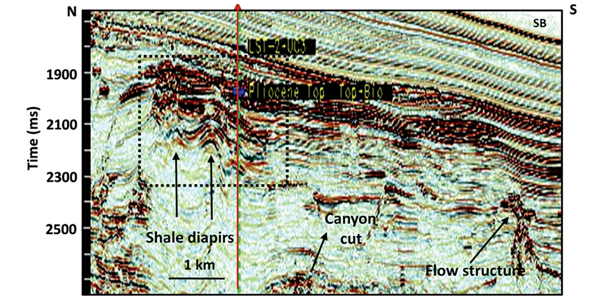
The seismic profile shown in Figure 1 depicts the superdeep Pliocene high amplitude seismic anomaly with typical bathyal geologic setting in the back drop. The anomaly was interpreted as an intricate strati-structural feature of hemipelagic siliciclastic fills in troughs formed as consequences to growths of conjugate flank shale diapirs. The feature was structured and morphed to its present form in an extensional shale tectonics regime, typified by episodic growth of diapirs and associated high angle normal faults, followed by late canyon erosional cuts. The Pliocene bathyal tectonic footprints of shale diapirs, mudflow structures and canyon-cuts are highlighted in the seismic section (Figure 1). The Pliocene fills were believed to be derived from the massive prograding Bengal fan which brought enormous amounts of siliciclastic sediments for dispersal of sands in the bathyal zone of the Bay of Bengal.

Pre-drill prospect appraisal

The prestack time and depth migrated 3D seismic data were used for prospect mapping and appraisal. Prestack depth migration was carried to improve imaging by ridding possible complications due to fast changing steep bathymetry and strati-structural complexity of the feature. PSDM, however, did not show noticeable changes over the PSTM except for marginal improvement in reflection amplitudes and structural details including fault plane definition (Figure 2).

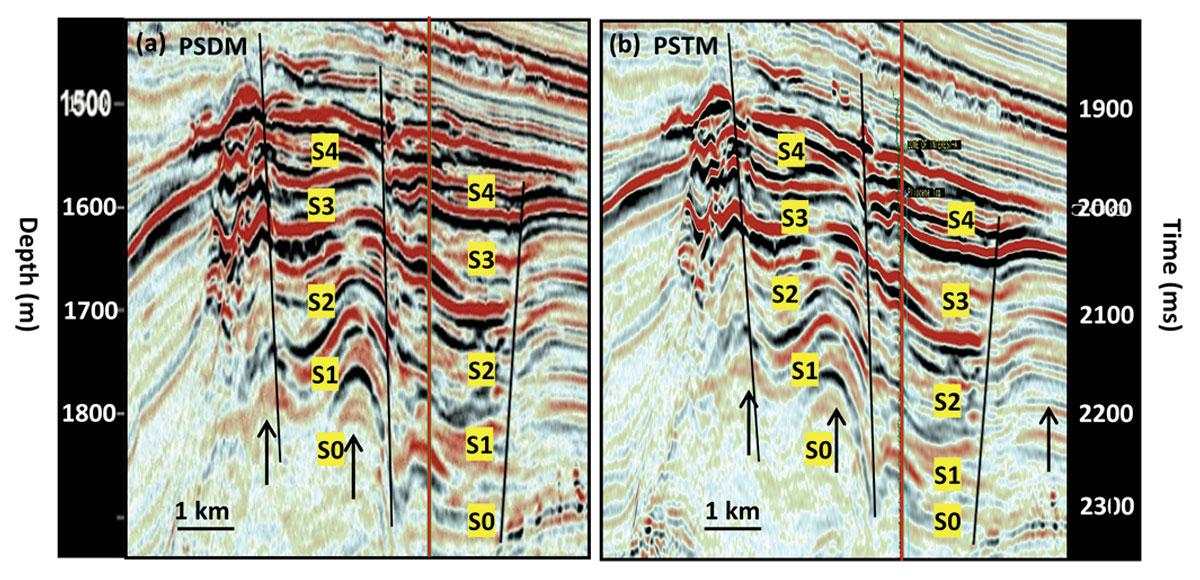
Five trough-filled seismic sequences were initially identified within the prospect, S0 to S4 (Figure 2). The strong seismic amplitude events in the top two sequences S4 and S3 were interpreted as due to alternation of finer and relatively coarser clastic facies, while the underlying S2, S1 and S0 sequences were considered mostly shaley, as indicated by poor and patchy reflections. The high amplitude events in the top two sequences were prognosticated as hydrocarbon bearing layers in sands brought and dispersed by the massive Bengal fan. The considerable areal extent of the seismic anomaly of nearly 20 km2 and multiple layers of sand reservoirs encased in thick shales of source rock, coupled with shallow drilling target of 500 to 700 m below the sea bottom, made it an attractive prospect to explore for hydrocarbon potential in the bathyal zone. The well was drilled on a small relief on the hanging wall of a fault, a locale proximal and updip to basinal source, considered favorable for hydrocarbon accumulation.

Post-drill analysis

Predicted and the actual; inconsistencies between seismic and log

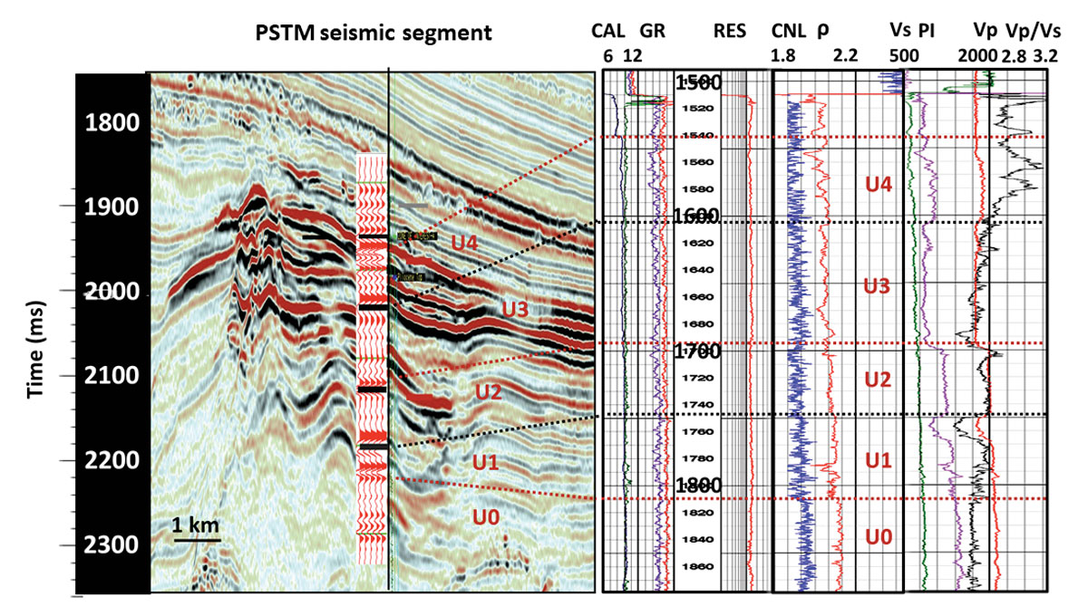
Drilling corroborates the seismic sequences but without the predicted reservoir sands, despite penetrating more than 400 m of sedimentary section of monotonous mudrocks through the seismic anomaly. The sonic and density logs, however, show noticeable impedance contrasts due to facies change within the thick mudrocks, which help identify five distinct rock units U0-U4 that can be classified as shale, claystone, mudstone and siltstone facies based on velocity and density values. The log rock units U0-U4 broadly validates the pre-drill interpreted seismic sequences S0 to S4 and is illustrated in Figure 3 which displays the log derived impedance curve interspliced between PSTM and PSDM seismic sections. Without well velocity data, the seismic-towell tie is attempted through the PSDM depths. Log depths of units are transferred onto the PSDM which shows reasonable match (for the upper ones), and the linked seismic reflection events are charted onto the PSTM section. Reflection times picked from PSTM are then used to compute seismic interval velocities for comparison with sonic velocities, to validate correlation of the seismic sequence boundaries with the geologic units at the well.

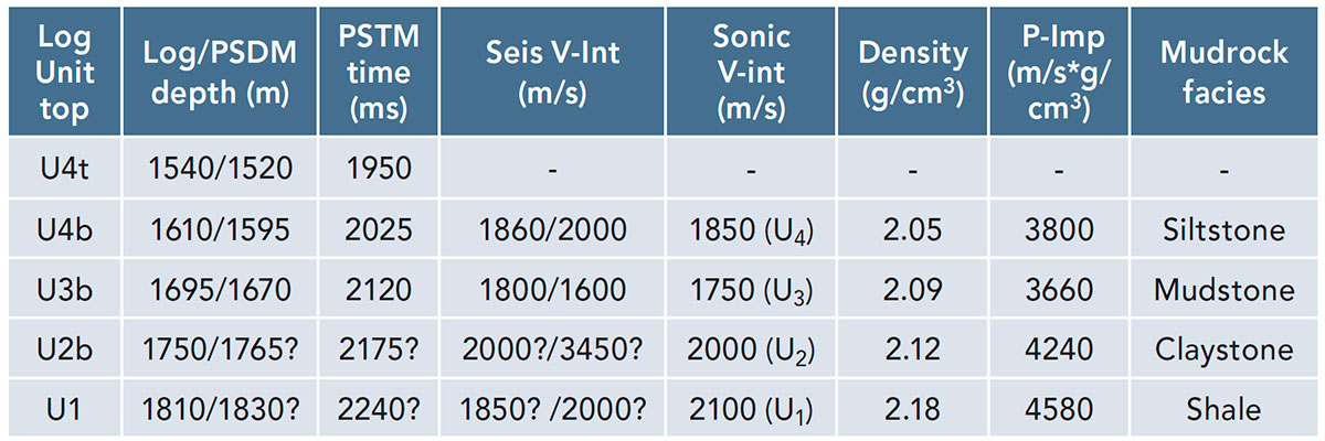
Table 1 is a comprehensive list showing the correlation between the log rock units and seismic reflection events along with the log and PSDM depths, corresponding PSTM times, seismic and sonic interval velocities, their densities and impedance contrasts. The PSDM depths match the log depths for the upper sequences with acceptable discrepancies of 15-25 m but are highly questionable for the lower sequences due to poor reflections. Seismic velocities are computed for both the log and seismic (PSDM) depths from the corresponding PSTM times for comparison with sonic velocity. The comparable sonic and seismic velocities for the upper log units U4 and U3 validate the sequence boundaries of S4 and S3, the main objects under study (Table 1 and Figure 3). However, correlativity of lower sequences U2 and below is unreliable in seismic as exact time cannot be picked due to absent or poor reflections. One such time, however, picked as a trial for the supposed reflection from U2 bottom, provides an unreasonable velocity (3450 m/s) for a claystone unit and the huge mismatch with sonic velocity (2000 m/s) proves the inaccuracy of the pick and the ambiguity of the correlation. The figures with question marks in Table 1 are the uncertain ‘best-guessed’ time and depth picks in PSTM and PSDM and the computed unrealistic velocities.

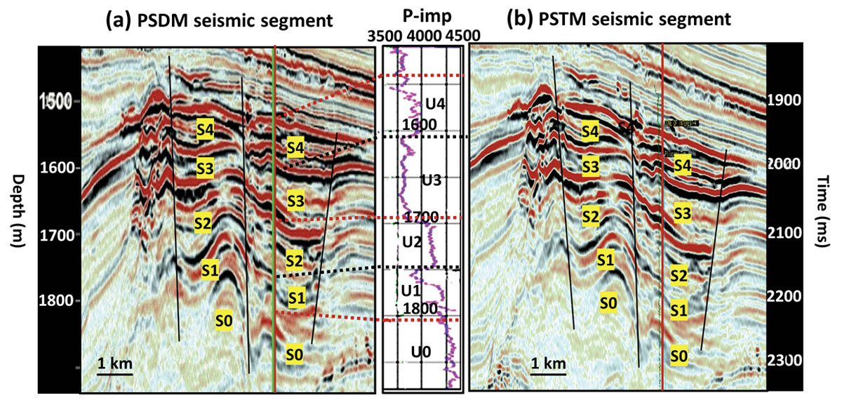
Examination of reflection events within the validated seismic sequences corresponding to rock units U4 and U3 (Figure 3 and Table 1), and for unit U2 reveals inconsistencies between the logged rock properties and their seismic response. For instance, strong contrasts seen in logs at the bottom of U2 and to somewhat lesser extent below, are represented by poor or no reflection events in seismic. On the other hand, the seismic high amplitudes seen within U3 and U4 are without analogous matching contrasts in logs. Interestingly, these high amplitude seismic events corresponding to the prime exploration targets for hydrocarbon sands, as it transpired, were caused not by customary impedance contrasts but due to other reasons. This had misled interpretation and resulted in a pitfall. Synthetic seismograms and prestack gathers are computed to probe in detail the reasons for the discordance.

Discussions

Synthetic seismogram and seismic calibration

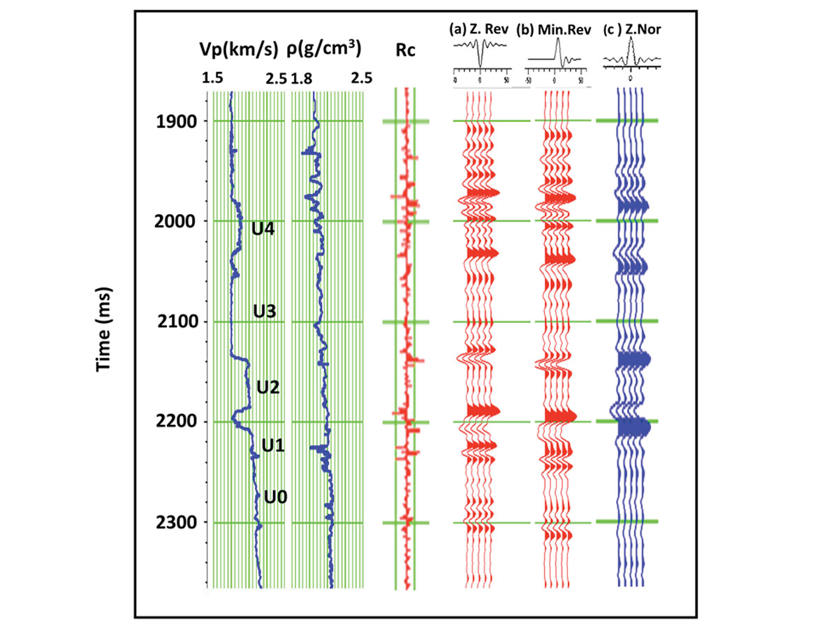
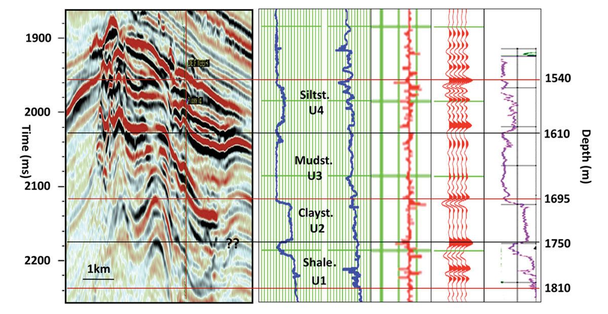
Three types of wavelets are used for computing the synthetic seismograms (Figure 4), however, the zero-phase, high bandwidth, and reversed polarity (SEG) wavelet provided the best synthetic match with the seismic data. The PSTM segment with spliced synthetic seismogram, along with the suite of logs with rock units marked, illustrates the well-seismic calibration (Figure 5). For better clarity and comprehension, composite display of zoomed version of PSTM seismic with a panel entailing the log velocity, density, reflectivity, computed synthetic traces and impedance curves is shown in Figure 6. It displays the variations clearly in each of the rock and seismic parameters, that influence the seismic response and help better analyze the reasons for the discordances between logs and seismic as discussed below.

i) Significant impedance contrast in log at U2 bottom showing poor seismic response.

The U2 is a relatively high impedance claystone unit with significant and discrete (sharp) contrasts at the top and bottom (Table 1 and Figure 5). While the top is expectedly represented by a strong reflection (red), strangely, the bottom response is not discernible in seismic, though the model synthetic trace shows strong responses. The time picked on a weak reflection (black), best-guessed to correspond to the bottom log contrast, as stated earlier, shows an unusually high seismic interval velocity (Table 1, and figures 5 and 6), and ascertains absence of valid reflections for the contrast at the bottom of U2. Despite good quality data, the absence of reflection from a strong acoustic impedance contrast in logs seems strange and inexplicable. However, scattering due to isolated and localized heterogeneous facies with inadequate small Fresnel zone may be plausible for the poor seismic imaging, even in the PSDM sections.

ii) High amplitude events within U3 and U4 showing poor impedance contrasts in logs

The bands of seismic high amplitudes within U3, the exploration objectives for hydrocarbon sands, belong to a low-velocity mudstone unit, characterized by near-flat sonic and density logs without noticeable variation. Yet, surprisingly, high amplitude events are seen near U3 base, though the synthetic trace shows expected weak responses (Figure 6). The reflections, nevertheless, seem to be genuinely from geologic strata as their correlation and continuity can be traced up dip, across the fault, to the foot wall side of the prospect.

Similar to U3, more and stronger reflection bands within U4 (Figure 6) also show little correspondence to the impedance contrasts in logs. Though the velocity curve is fairly even, the density log shows moderately pulsating variations that influence impedance contrasts to create a number of closely spaced thin-bed reflections as indicated by the model trace. A possible explanation for the high amplitudes within U4 may be the constructive interference of several such thin-bed weak reflections resulting in strong-reflection composite event. This also entails problems in detection of proper phase, polarity and arrival time of reflections, impeding one to one correspondence with log events. However, the occurrence of large variations in V_P /V_S log plot, corresponding to the high amplitude events within U4 (Figure 5), led to probe the likely role of V_P /V_S in causing the high amplitudes by modeling and studying an elastic gather.

Elastic gather modeling

The prestack elastic gather is modeled using the compressional- and shear-wave velocities, V_P and V_S, and the density ρ, to examine the amplitude variation with offset (AVO) pattern (Figure 7). The parameters are picked on the log at a point of maximum positive V_P /V_S contrast (shown by arrow) within U4, and the values and log curves are displayed in the text of the figure. The synthetic prestack gather shows the expected weak positive amplitudes in the near traces due to marginal P-impedance contrast but steeply increasing amplitudes around mid-offsets, and ending with strong amplitudes at the far traces. Once stacked, they would show high amplitudes in the full-stack seismic section and explain the strong reflections within U4 despite minor contrast in P-impedance.

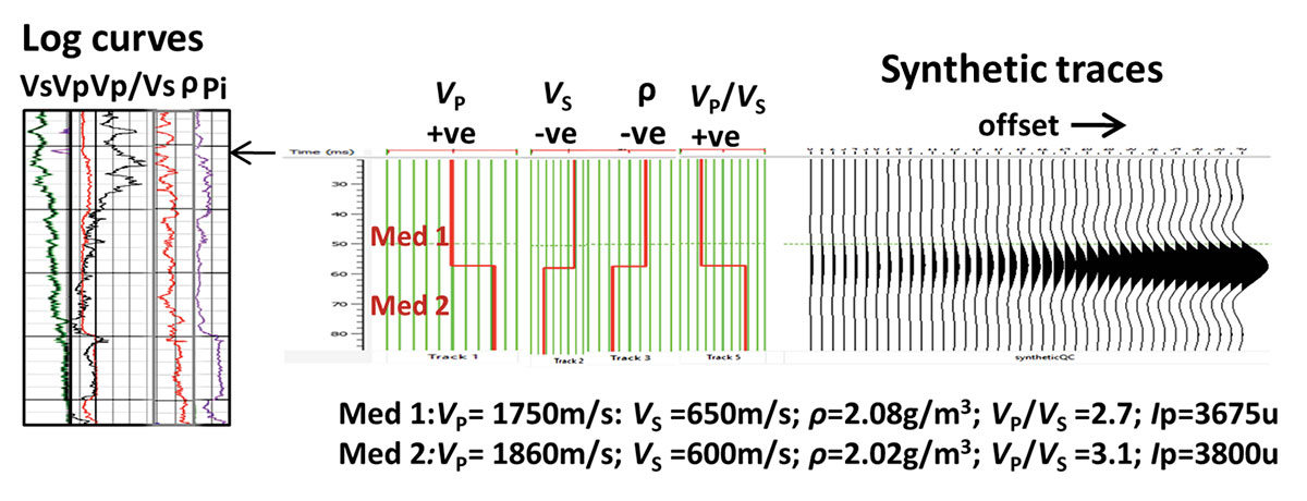
Ostrander (1984) had demonstrated amplitude increase with offset for a medium having positive contrast in P-impedance and Poisson’s ratio, which gets more pronounced with larger contrasts in Poisson’s ratio. Poisson’s ratio is reportedly large for shallow, unconsolidated, brinesaturated mudrocks in offshore deep waters, and high contrasts in their magnitude, due to facies changes within mudrocks, are likely to show strong amplitudes in stack sections without the requisite contrasts in P-impedance.

However, the occurrence of high amplitudes in U3 without impedance contrasts cannot be explained by contrasts in Poisson’s ratio as the V_P/V_S curve within the unit is seen flat. It may be mentioned that for the seismic amplitudes to result without noticeable contrasts in impedance, as in the present case, it is possible that attenuating layers in the subsurface could be their source, as has been reported by Gibson (2008) and Lines et al. (2012). Further investigating this possibility was outside the scope of the present exercise due to unavailability of the required information but could be taken up in the future.

The pitfall

The fact that the high amplitude events are not related to hydrocarbon sands but to facies changes within the mudrock matrix caused the pitfall. The amplitude change with offset in Figure 7 is not typical AVO response for hydrocarbon sand, but nevertheless, patterns similar to hydrocarbon sands are possible from diverse configurations due to wide variations in matrix and fluid properties of young siliciclastic rocks deposited under differing geologic setting. Several examples of high amplitude Pliocene high amplitude anomalies in offshore East coast of India are cited (Nanda, 2017), illustrating effects of varying rock matrix and fluid properties on AVO attribute patterns. AVOs, apparently similar to genuine hydrocarbon patterns, but caused by matrix changes in mudrocks, can thus be risky of being misinterpreted for hydrocarbon sands and need cautious analysis. Pliocene-Pleistocene seismic strong amplitude anomalies in bathyal environment can be especially tricky for AVO interpretation, and inability to predict the rock and fluid properties unambiguously can result in seismic interpretation pitfalls.

Conclusions

1. The high amplitude seismic events in U4 are caused mainly by large VP /VS contrasts in matrix within the mudrocks and not by P-impedance contrasts, which led to the pitfall.

2. Small changes in density within the mudrocks generated a number of thin-bed reflections which interfered constructively and created composite seismic events of high amplitudes.

3. AVO for high amplitude seismic anomalies, especially in young Pliocene/ Pleistocene of bathyal environment, can be misleading as the amplitude increase with offset can be due to contrasts in Poisson’s ratio within mudrock matrix and unrelated to fluid.

4. Reason for poor reflection from U2 bottom having strong impedance contrast in logs is unclear. However, scattering due to heterogeneity and inadequate Fresnel zone width may be reasons for the poor image.

5. Seismic interpretation pitfalls can happen even with good quality 3D PSTM and PSDM data due to geologic problems and innate seismic limitations.

Acknowledgements

My sincere thanks are due to Srivatsa Das, GGM (Geology), MBA basin, ONGC and Servesh Mallick, GGM (Petro physics) KDMIPE, ONGC, for the seismic and log data.

I am thankful to Satinder Chopra, TGS, Calgary, for his help with the computed models and other useful suggestions.

I am grateful to Oil and Gas Corporation Ltd., India for permission to publish the paper.