Anisotropic Pre-Stack Depth Migration

Seismic anisotropy is the variation of velocity with direction. This phenomenon may affect time-to-depth conversions of seismic data which, in turn, will result in incorrect images of subsurface structures. This misrepresentation can seriously alter the location of exploration targets. By studying seismic anisotropy, one can better assess a play target, thereby reducing the risks and costs involved. The main causes of seismic anisotropy are due to aligned mineral grains, aligned cracks, aligned crystals and periodic thin layering [Helbig, 1994]. The effects due to periodic thin layering are most pronounced in layered clastic sequences, specifically shales or interbedded shales and sandstones. It is known that the majority of sedimentary basins contain considerable amounts of shales and are also the main location of hydrocarbon reserves [Schoenberg, 1994; Sayers, 1994; Hornby et al., 1994]. Banik (1984) discovered a strong correlation between the presence of shales and a measured velocity anisotropy in North Sea sediments. It has been shown by many researchers that shales exhibit transverse isotropy (TI), with the symmetry axis perpendicular to bedding, when probed by seismic energy with wavelengths that are greater than the thickness of the layers [Johnston and Christensen, 1995; Backus, 1962; Postma, 1955; Levin, 1979; Schoenberg, 1994]. The difference between velocities perpendicular and parallel to bedding is significant, increasing with the degree of anisotropy and can be as much as 30% in shales [Backus, 1962; Berryman, 1979; Levin, 1979; Jones and Wang, 1981; Banik, 1984; Gaiser, 1990; Sayers, 1994; Hornby et al, 1994; Kebaili and Schmitt, 1996]. This can result in apparent, residual depth structures of several hundred metres for targets at several kilometres depth. Velocity anisotropy is also likely to exist in interbedded shales and sandstones in the Rocky Mountain Foothills, where folding and faulting can thrust these stratigraphic horizons, often at steep dip angles, to the surface. These dipping layers are expected to induce changes in velocity which result in traveltime anomalies in the seismic data [Crampin, 1977; Gaiser, 1990].

Physical models, representative of structures found in the Foothills of central Alberta and incorporating anisotropic material (phenolic laminate), have been used to demonstrate the pull-up effects of anisotropy due to a steeply dipping shales. These physical models, initially described by Leslie and Lawton (1998a), are extremely useful for assessing effects of anisotropy on seismic images since the velocities, anisotropic parameters, dip angles, and the exact location and geometry of the thrust sheets are known a priori. This allowed us to determine if the effects of anisotropy, particularly transverse isotropy, significantly affect isotropic migration results. The results of the first model were conclusive [Leslie and Lawton, 1998a]: anisotropy is a significant effect, contributing to both lateral and depth positioning issues, and that isotropic migration is not able to properly account for these effects. A second model, made completely of Phenolic laminate, is considered to be a more geologically representative model as it better approximates the structures found in the Alberta Foothills. Numerical modelling performed on the second mod el indicates that the magnitude of the anisotropy of dipping strata affects travel times Significantly, with distortions in the stacking velocity field greatest for intermediate dips [Leslie and Lawton, 1998a].

Pre-stack depth migration was performed on both physical models using both isotropic and anisotropic velocity models. The difference between isotropic and anisotropic migrations is in the code used (courtesy of Kelman Technologies Inc.), the traveltime generator for the anisotropic, Kirchhoff, pre-stack depth migration has been altered so that anisotropic group velocities are used to propagate the wavefronts. In the isotropic case, a point on the wavefront propagates normal to the wavefront using the local velocity. In the anisotropic case, a point on the wavefront propagates radially outwards from the sourcepoint at the group velocity, which may be oblique to the wavefront normal [Vestrum et al. 1998].

Physical Model 1

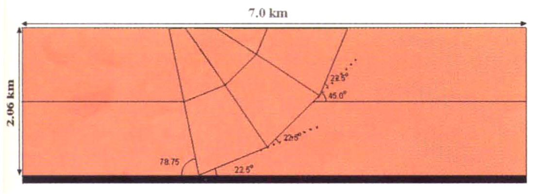
A 1:10 000 scale model of an anisotropic thrust sheet was constructed in the physical modelling laboratory of the Department of Geology and Geophysics at the University of Calgary (Figure 1).

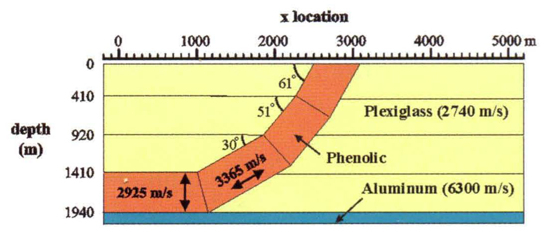
The model mimics structures found in the central Alberta Foothills. Phenolic laminate, consisting of layers of cloth which have been glued together with epoxy, was used as the an isotropic material because it has well understood elastic properties [Cheadle et al., 1991]. A simulated thrust sheet was constructed such that the corresponding fast and slow velocities were V_slow = 2925 m/s and V_fast = 3365 m/s [Cheadle et al., 1991]. The Thomsen (1986) anisotropic parameters were determined to be δ = 0.081 and ε = 0.150 [Cheadle et al ., 1991]. The surrounding isotropic medium was made of Plexiglass, which has a measured velocity of 2740 m/s [Cheadle et al., 1991]. The marker of interest was the reflection from the horizontal, aluminum base of the model, at approximately 2 km depth (scaled), below the thrust sheet.

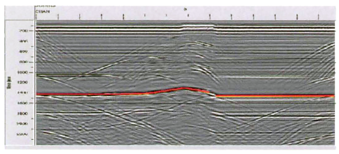
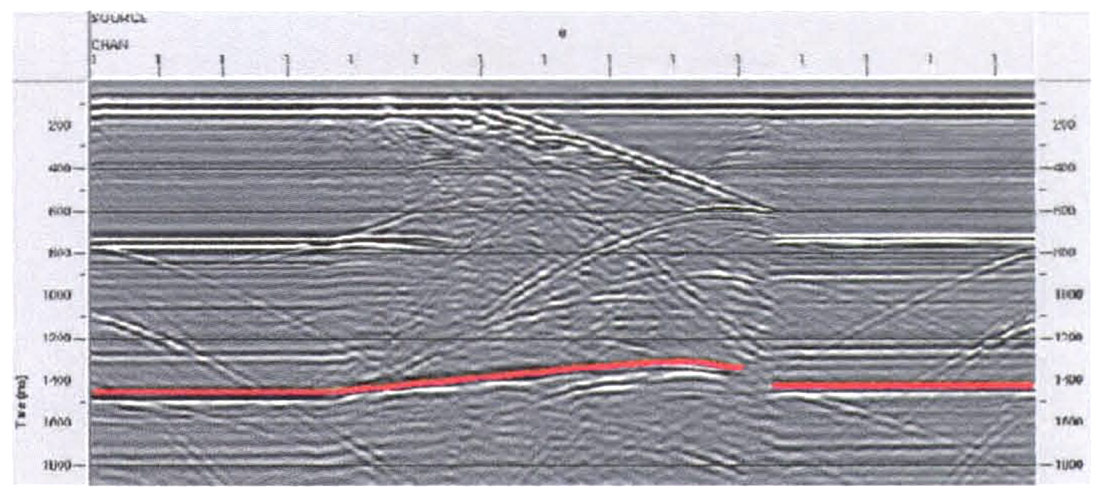
Results of the 2-D, zero-offset, ultrasonic survey across the model show an apparent structure in this basal reflector, with an amplitude of approximately 100 ms (Figure 2). After eliminating the isotropic velocity pull-Up from the data, due to the larger volume of faster material in the thrust sheet, the residual anomaly due to anisotropy is 50 ms. This translates into a residual depth structure of approximately 100m, which is the magnitude of structures that are considered prospects in the Foothills. Hence the effects of anisotropy due to steeply dipping clastics are represented and significant in the seismic data obtained from the physical model.

Pre-Stack Depth Migration – Model 1

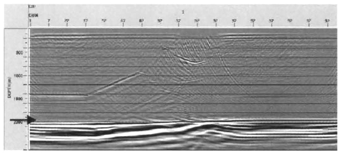
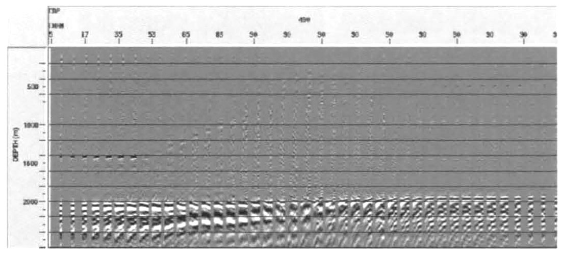
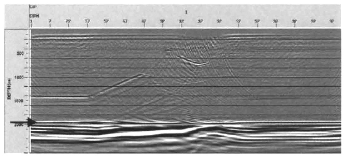
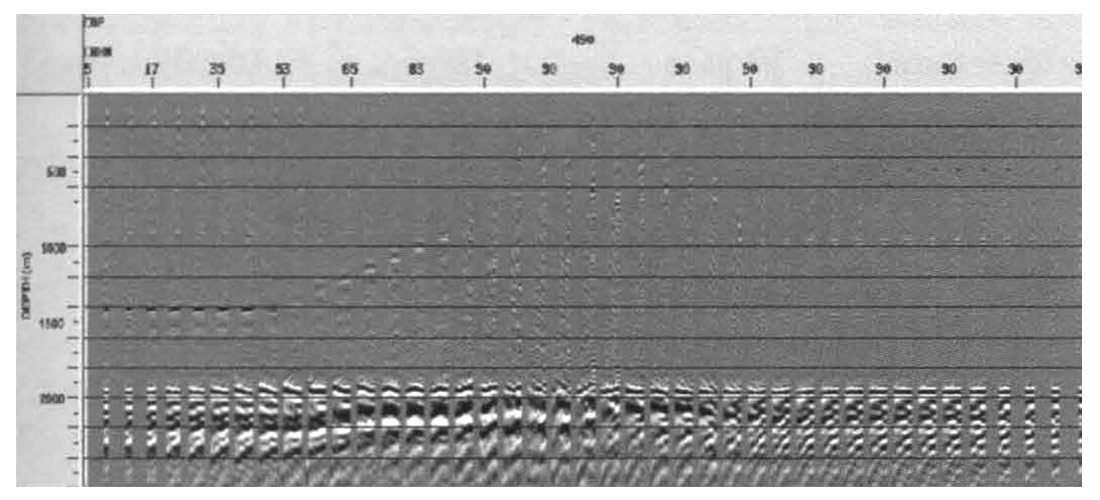
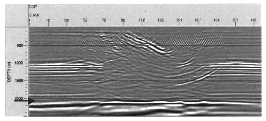
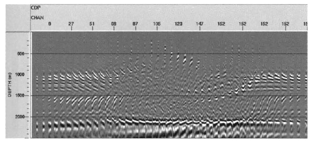
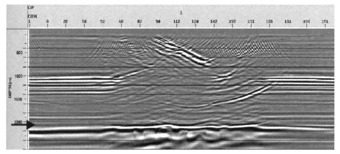
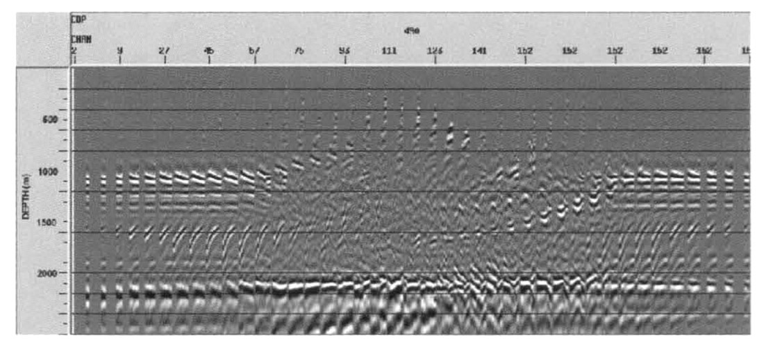
The physical model data were processed as follows: mute; prestack depth migration (isotropic and anisotropic); scale; and filter (band pass Ormsby 8-12, 50-60 Hz). The data were first migrated isotropically, with a velocity model built using the constant fast velocity of the thrust sheet and its actual spatial location, for the migration. The results of this migration are shown in Figure 3 and the associated depth gilthers in Figure 4 (near offsets on the right and far offsets on the left). The continuity of the basal reflector is good; however, it is located too far in depth under the thrust sheet. In addition, the gathers in this location indicate that the migration velocity is too low and should be increased, in doing so, the reflector would be pushed even farther in depth, which is incorrect.

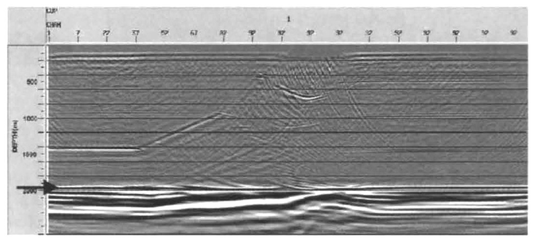
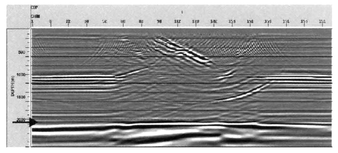
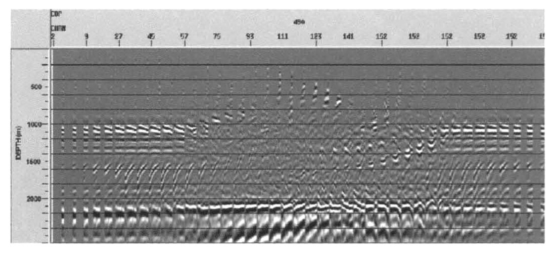
The second isotropic velocity model used a horizontal velocity gradient in the thrust sheet, grading from the fast velocity of the Phenolic in the top right comer of the thrust to the slow velocity in the flat lying Phenolic in the bottom left, in attempt to account for the anisotropy of the Phenolic material. The result is a correctly placed reflector, under the thrust sheet, with the continuity of the reflector somewhat compromised (Figure 5). The depth gather results indicate that, although the reflector is correctly located in depth, a faster migration velocity should be used to correctly migrate the data (Figure 6). This would also be incorrect, according to the known physical model.

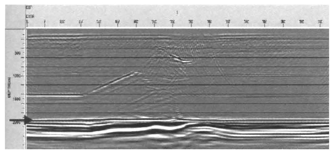
The only way to eliminate the discrepancy between correct depth and residual moveout on image gathers is to use anisotropic pre-stack depth migration. By using the correct velocity model, and all the correct parameters (δ, ε and dip) from the physical model, one obtains a correct depth image of the original model (Figure 7) which is supported by its associated depth gathers (Figure 8). Reflector continuity is maintained, it is correctly located in depth and events within the depth gathers are flattened. Hence, all the discrepancies from the isotropic depth migration process have been eliminated. It should be noted that the small amount of residual moveout in the depth gathers is associated with the velocity model building process. The migration velocity model is built in time. However, the physical data, measured from the model, are measured in depth, and the conversion from depth to time in the velocity model building process introduces small irregularities into the velocity model and, subsequently, in the migration. In conventional migration, the depth model is not known, thus the velocity model must be built deterministically.

Physical Model 2

Another 1:10 000 scale model of an anisotropic thrust sheet was constructed in the physical modeling laboratory (Figure 9). The model is comprised completely of Phenolic laminate with slow and fast velocities of V₂ = 2925 m/s and V₃ = 3365 m/s, respectively, and δ = 0.081 and ε = 0.150 [Cheadle et al., 1991; Thomsen, 1986J. The resulting degree of anisotropy is 13%. The surrounding flat layers are also made of Phenolic. The marker of interest was again the reflection from the horizontal base of the model, at approximately 2 km depth (scaled), below the thrust sheet. This model did not have an aluminum base to it.

The 2-D, zero-offset, ultrasonic survey data are shown in Figure 10. The amount of pull-up is less than 100 ms since the surrounding isotropic material had been replaced with the higher velocity Phenolic laminate, compared with lower velocity Plexiglass in Model I. Hence the velocity contrast is less compared to the first model, resulting in a smaller velocity anomaly, but one which is caused entirely by velocity anisotropy.

Pre-Stack Depth Migration – Model 2

The physical model data were processed using a mute, pre-stack depth migration (isotropic and anisotropic), scale and filter (bandpass Ormsby 8-12, 50-60 Hz). For comparison purposes this model was first processed isotropically, using a gradient velocity model. The base of the thrust was defined and a horizontal velocity gradient was applied to the dipping part of the thrust: grading from the fast velocity of the Phenolic in the top right corner to the slow velocity of the Phenolic in the flat lying layers, in the bottom left. The resultant isotropic depth migration is comparable to the results of the first model (Figure 11). The basal reflector is correctly located in depth, with some minor structure present; however, the depth gathers exhibit considerable residual moveout which indicates that a higher velocity should be used to properly migrate the data (Figure 12).

It is worthy to note that the continuity of the basal reflector is compromised because the model does not have an aluminum base. Since the model is sitting on a table top, thus going from a high velocity medium to a slow velocity medium, there is a negative impedance contrast at the base of the model. Also, there is a multiple (positive impedance) which constructively interferes with the basal reflector, resulting from the horizontal seam, halfway down the model, at approximately 1 km scaled depth. Thus the reflector is very strong in the middle of the section and weak at the edges (Figure 11).

Data from the second model were then migrated anisotropically This velocity model consisted of the definition of the thrust base, the actual parameters of the model (slow P-wave velocity, δ and ε) and a continuous definition of dip through the thrust sheet and across the model. No distinctions were made between the different blocks of dipping Phenolic as the thrust sheet was modelled as having continuous, smooth curvature. The basal reflector is correctly located in depth, although it is severely distorted (Figure 13). The gathers are comparably distorted as well (Figure 14). Given that the input model linearly interpolates the dips between defined values, whereas the actual model has distinctly dipping sections, the results are not surprising. Thus the input model is sensitive to the dips defined within it.

In the final anisotropic velocity model, each distinct, dipping section of Phenolic was correctly located, with appropriate dip as well as all the correct parameters of the physical model. The result is a correct depth section with good reflector continuity, correct reflector location and flattened events on the depth gathers (Figures 15 and 16). Again the gathers are subject to small depth-time conversion errors, as was noted in the results of the first physical model (Figures 7 and 8). Thus, the same sensitivity to the model building process is also present in the second physical model data.

Discussion and Conclusions

Physical models are very useful for the study of seismic anisotropy. Since all the necessary parameters of the model can be determined, the data provided by the model are ideal for the testing of processing software, in particular, migration routines. In this study, it has been demonstrated that isotropic, pre-stack depth migration is limited in its ability to correctly migrate data from the anisotropic physical models, as it leads to discrepancies between the correct reflector depth and the residual moveout in image gathers. The testing completed in this study indicates that conventional pre-stack depth migration is not able to properly compensate for the effects of TI, and the results verify that anisotropy cannot be accounted for using isotropic velocities. Therefore, we conclude that anisotropic, pre-stack depth migration is required to properly process seismic data from these models and, in general, data from foothills environments.

Acknowledgements

We would especially like to thank Kelman Technologies Inc. for the use of their pre-stack depth migration algorithm used in this study. Also to thank Ron Schmid and Rob Vestrum for their assistance and insight into this work.

We also gratefully acknowledge the financial support for this work provided through the sponsors of the Foothills Research Project (FRP) and the Natural Sciences and Engineering Research Council (NSERC) of Canada. Support for J. Leslie from NSERC, SEG and CSEG scholarships is also acknowledged.