Another Look at MEMS Sensors… and Dynamic Range

In an October 2003 CSEG RECORDER article, Tessman and Maxwell discuss the importance of vector fidelity in full-wave recording and the key design elements in achieving good fidelity. One important design element relates to tilt measurement and the proposed need for a sensor to be force balanced against gravity. Figure 2 of their paper addresses the issue of dynamic range as a function of tilt and creates comparisons among the VectorSeis‚ MEMS sensor, geophones and MEMS sensors without gravity compensation. This figure is, at best, misleading and fails to present the comparisons that are relevant.

In this paper, the issue of dynamic range versus sensor tilt is revisited and relevant comparisons produced. Other facets of MEMS system behavior important to the user are also addressed.

MEMS Sensor Designs

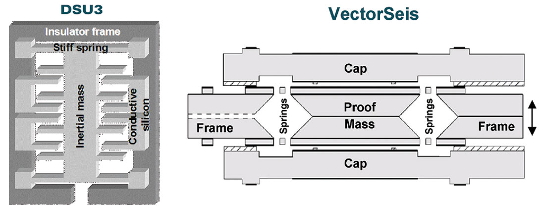
MicroElectroMechanicalSystem (MEMS) sensors provided to the seismic industry by Sercel (DSU3) and Input/Output (VectorSeis) have two principal components, a silicon micro-machined accelerometer and a custom designed, mixed-signal, application-specific integrated circuit (ASIC). However, the accelerometers employed have fundamentally different designs as indicated by the diagrams in Figure 1.

In the following we shall look at some simplified diagrams of DSU3 accelerometers but otherwise not pursue design details. Such matters are best left for the equipment manufacturers. From a user perspective there are, however, some key sensor behaviors related to design that are deserving of attention. These include: (a) impact on dynamic range, (b) sensor power requirements, (c) sensor noise levels, (d) data overscaling/recovery and (e) sensor testability. We shall consider each of these issues with the primary focus on dynamic range.

Accelerometer Comparison

With the VectorSeis sensor, each of the three orthogonal accelerometers is identical with each proof mass centered using an electrostatic force to balance the impact of gravity. Given such centering, there is no tilt effect on the full scale of the analog to digital converter and thus the sensor can be deployed at any angle. This results in a flat instantaneous dynamic range versus tilt response as indicated in the Tessman et al article. A cost for this functionality is the need for additional power to electrostatically counteract the force of gravity.

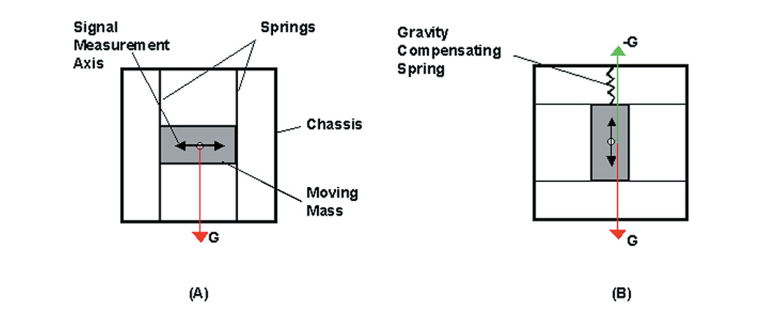
Figure 2 provides a simplified schematic diagram describing the horizontal and vertical accelerometers of the DSU3 sensor. The horizontal accelerometer has no compensative force against gravity(G) and the vertical component anticipates the gravity deflection in the fabrication stage and employs an auxiliary spring to naturally center the mass in the vertical position. With this design, part of the analog to digital converter’s full scale is taken up by the tilt-induced acceleration as will be described. The net result is that dynamic range suffers some decay as a function of tilt.

So a potential design trade-off is power consumption versus dynamic range. Regarding power consumption, the DSU3 sensor has minimal power needs requiring only 400 mW of power per three channels. Power requirements for the VectorSeis sensor are elevated, as expected, to accommodate force balancing but the specification is unpublished. Power is an extremely important issue as battery management is a significant factor in daily field operations where channel counts on multicomponent projects are typically more than triple that of conventional P-wave projects. Vibroseis, heliportable and cold weather operations only magnify this problem, increasing the importance of reduced power consumption.

Let us now look at the issue of sensor dynamic range versus tilt and consider the magnitude of loss in dynamic range for the DSU3 design.

Dynamic Range versus Tilt

It is by now well-known that MEMS sensors (DSU3 or VectorSeis) have a number of very desirable characteristics relative to their triphone ancestors. These include:

1. Direct digital output
2. Improved vector fidelity
3. Broadband linear phase and amplitude response
4. Low harmonic distortion Measurement of sensor tilt
5. Reduced power consumption

Because of the aforementioned variations in MEMS sensor designs, tilt has differing effects on the dynamic range of a sensor. Figure 2 from the Tessman and Maxwell paper (referenced in the introduction) showing dynamic range versus tilt comparisons is reproduced here as Figure 3.

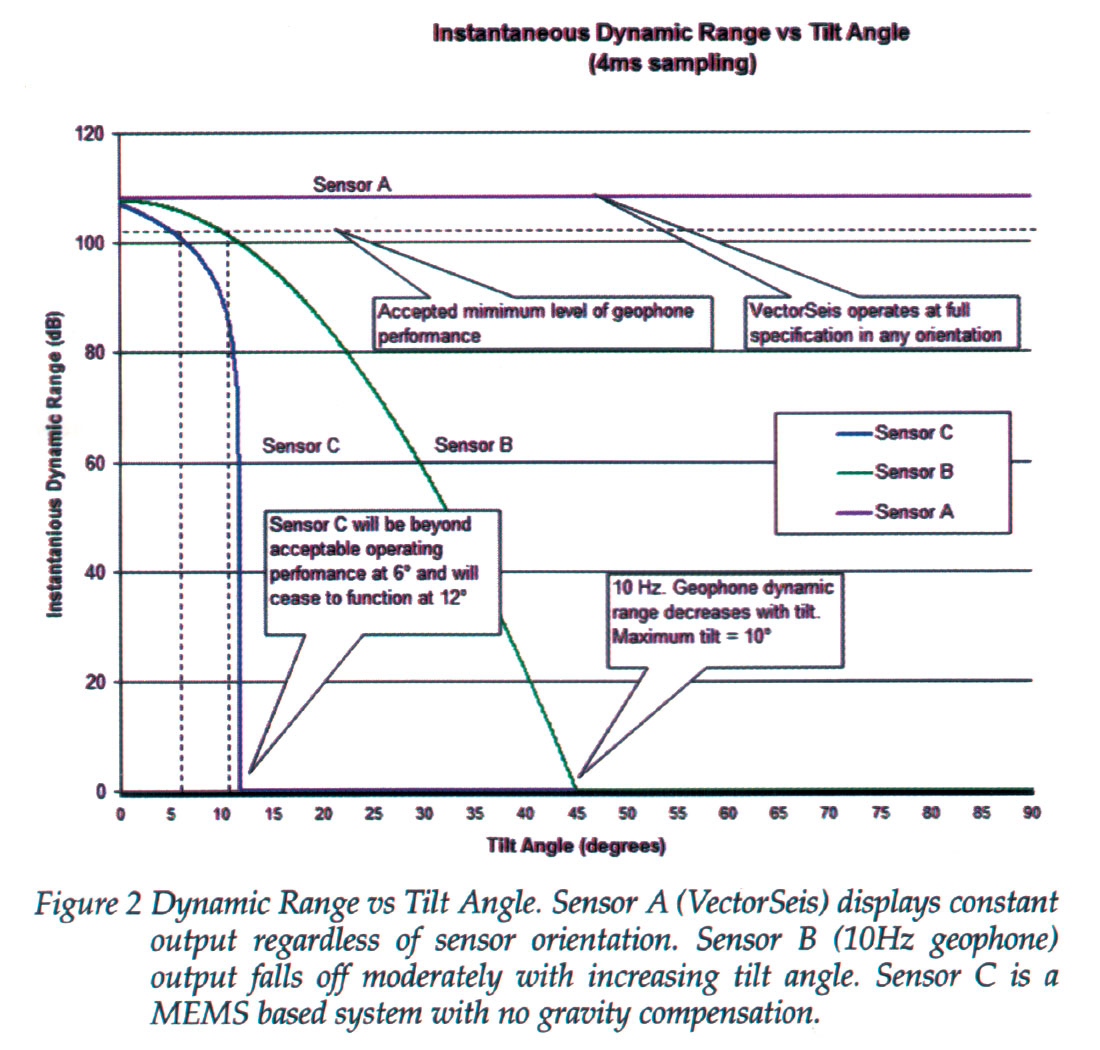
Referencing Figure 3, Sensor A (VectorSeis) does, in fact, provide constant output regardless of sensor orientation although the indicated level of 108 dB corresponds to 2 ms (not 4 ms) sampling according to published specifications. Second, both the zero-tilt value and decay of Sensor B (geophone) are erroneous. Conservatively, the dynamic range of a 10 Hz GS-32CT geophone is well above 110 db even at 10�� tilt. The real limitation for geophone output is the recording system, not the sensor. Figure 5 shows the corrected geophone decay curve.

Sensor C (assumed to be the Sercel DSU3 sensor) requires further discussion. Sercel provides for two scales of sensitivity, G1 and G2, with the G1 scale used exclusively. G1 has a larger full scale and is less affected by tilt than the G2 scale that was inappropriately used for comparison in Figure 3.

Since the horizontal and vertical accelerometer designs of the DSU3 sensor differ, a proper correction of Figure 3 must show decay curves for each. Figure 4 shows each of the elements tilted by an angle θ. With tilt, the gravity vector G can be resolved into two orthogonal components, G_o (orthogonal to the sensitive axis) and G_s (inline with the sensitive axis).

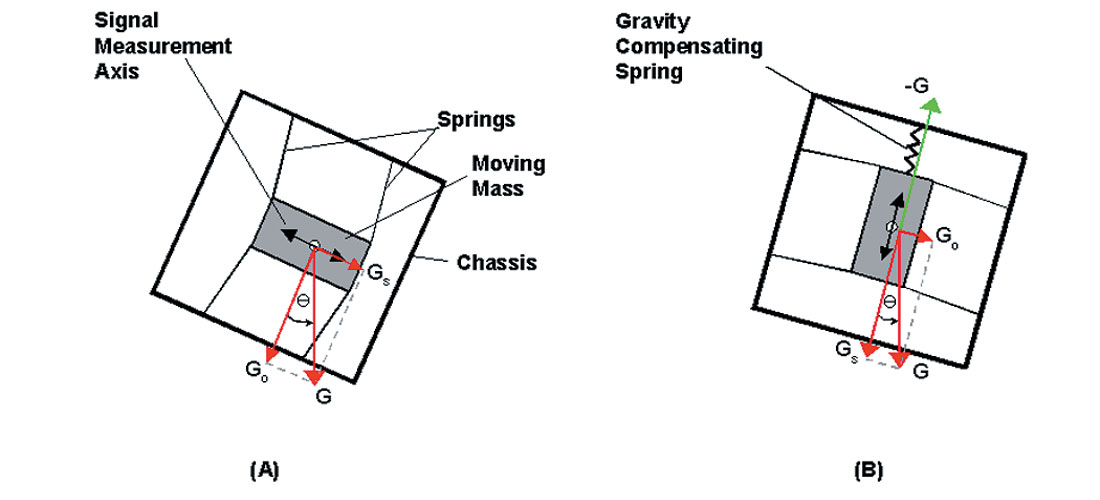
Referencing Figure 4(A), G_s = Gsinθ is the horizontal acceleration encoded by the A/D converter owing to tilt. When G_s = 4.5 m/sec² ~ .459G, the A/D converter is at full scale at G1 sensitivity and the converter is full with no remaining room for signal encoding. For the horizontal element this occurs at an angle, θ_HMAX, given by

θ_HMAX = sin^-1 (.459) ~ 27.3°

Using Figure 4(B), the vertical accelerometer sees a bias, B, given by

B = G_s – G
= Gcosθ - G
= -G (1-cosθ)

for a tilt of θ.

In this case, full scale (owing to tilt) is reached when the bias overdrives the sensor. This occurs when

B = -4.5 m/sec² ~ -.459G

or

θ_VMAX = cos^-1 (1 - .459) ~ 57.23°

So, the tilt angles for which no signal can be recorded are, in fact, quite different for the horizontal and vertical elements. Derivations of dynamic range decay formulae for the horizontal and vertical elements can be found in the appendix. These formulae, together with a geophone decay formula, are used to develop Figure 5, the corrected version of Figure 3.

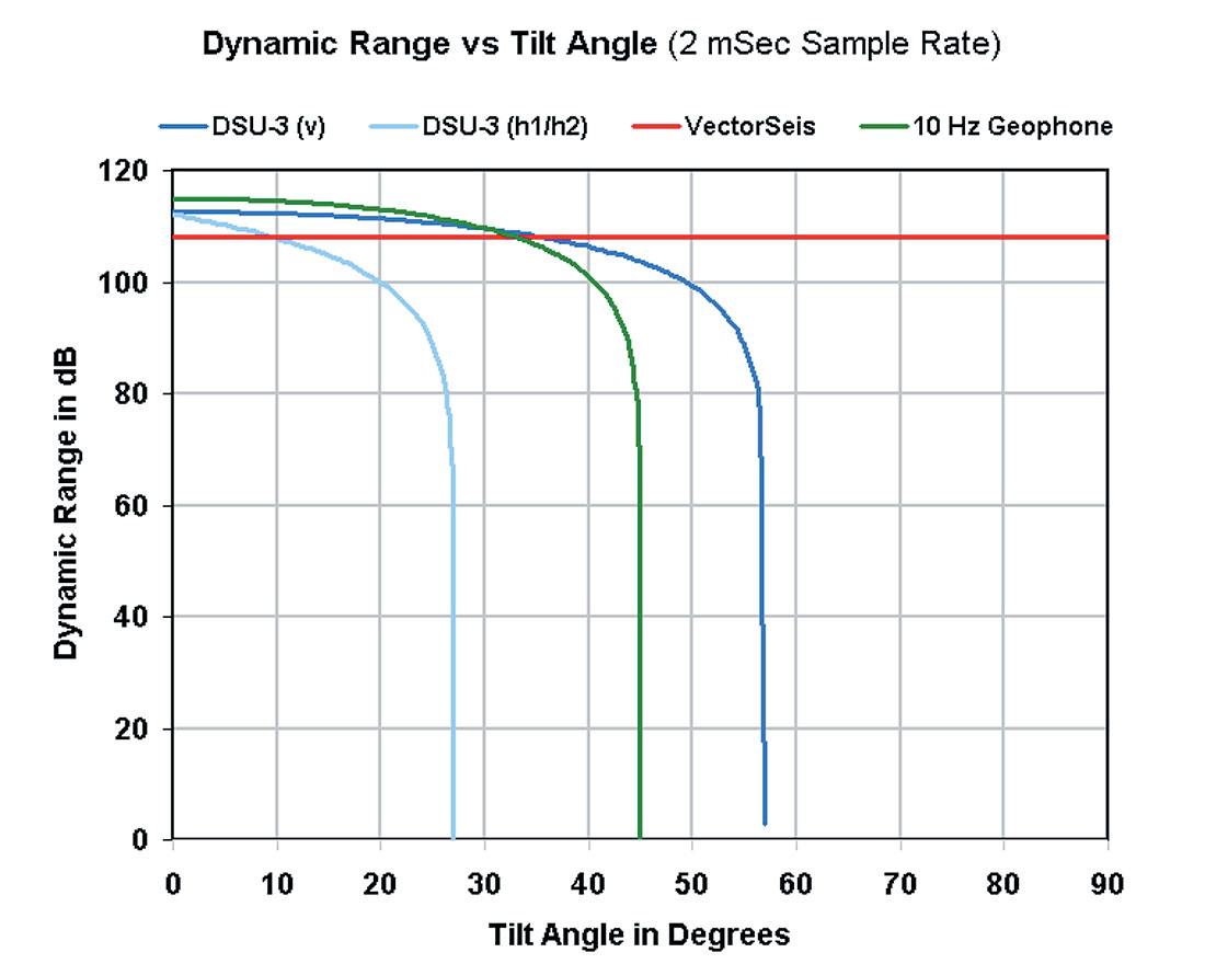
A cursory look at Figure 5 might lead one to conclude that there is a distinct advantage in using the VectorSeis sensor as its dynamic range is flat as a function of tilt. If we enlarge Figure 5 and restrict the tilt angle to 10 degrees (Figure 6) it becomes apparent that when the sensor is planted with less than 9 - 10 degrees of tilt the DSU3 has, at a minimum, the equivalent dynamic range as the VectorSeis sensor for a sample rate of 2ms.

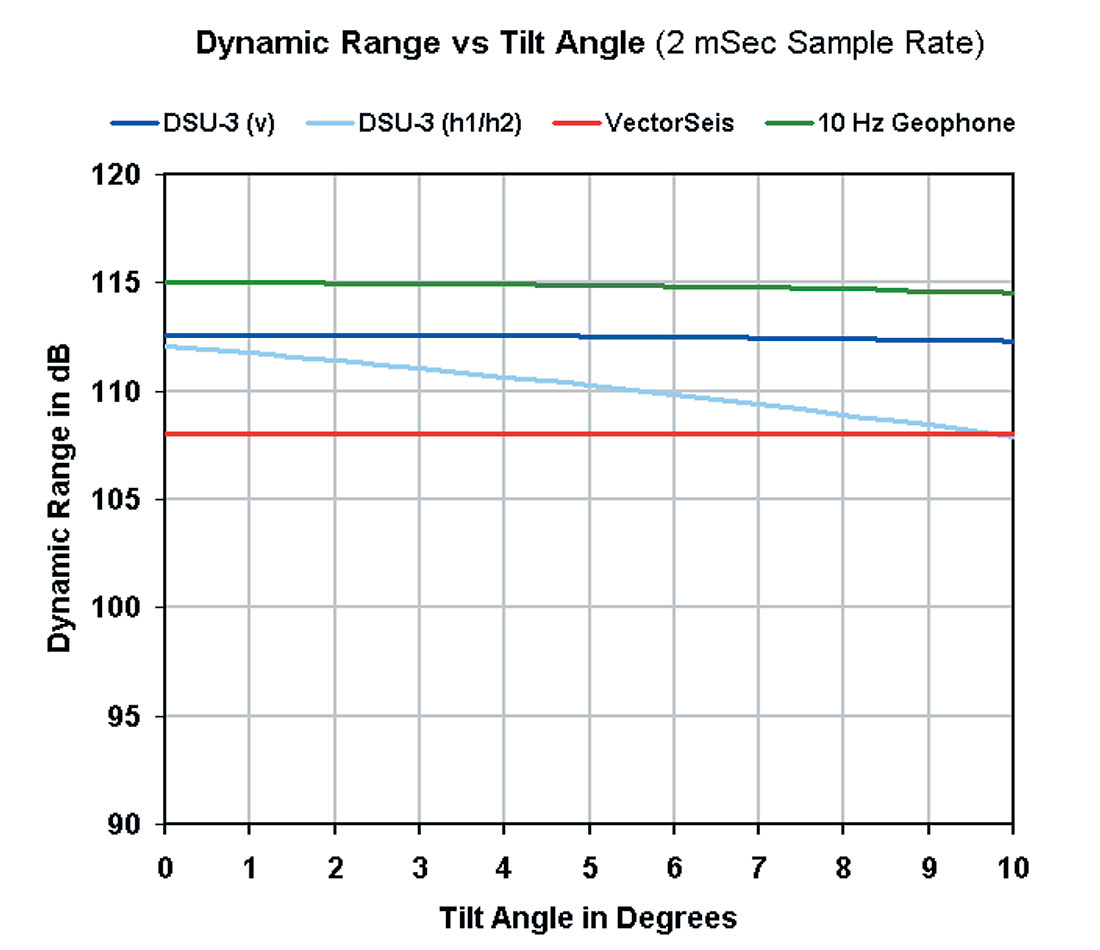
Note: The dynamic range calculations for each sensor type have utilized a “typical” signal maximum rather than the theoretical A/D converter maximum. For example, the VectorSeis theoretical maximum is ~ 0.335G while the “typical” maximum ( before overscaling ) is ~ 0.225G. In producing any device such as a MEMS sensor there will be some variability in characteristics such as achievable signal maxima. Also, tilt angles for which DSU3/VectorSeis “crossover” in dynamic range occurs varies slightly with a change in sample rate.

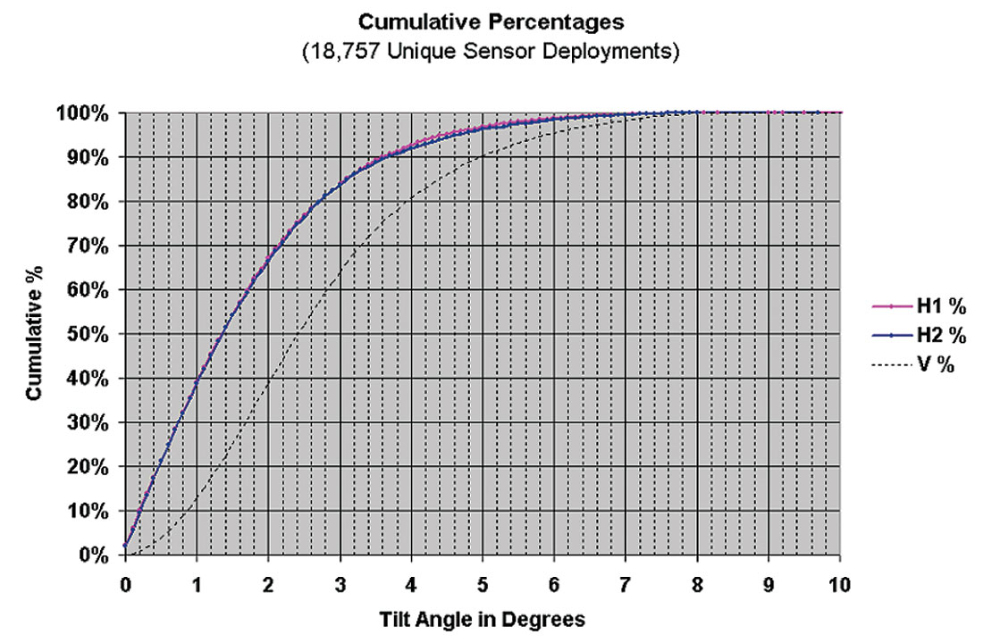
How realistic is it to expect MEMS sensors to be deployed with less than 9 - 10 degrees of tilt during land operations? Figure 7 shows the cumulative percentage distribution of tilt angles (horizontal and vertical) for over 18000 initial sensor deployments. These include both DSU3 and VectorSeis deployments over a three-year period. In normal operation, over 99% of sensors have less than 8 degrees (Veritas specification) of tilt upon initial deployment. Further, since tilts are reported in the recorder by the system, the small percentage of sensors that exceed this specification can easily be replanted. Our experience indicates that the need to deploy sensors at extreme angles is exceptional. Veritas tests of horizontal deployment of VectorSeis sensors indicated difficulties with coupling even with the use of sand bags. In the seabed environment, sensor tilt is less controllable and sensors that are force balanced against gravity may be attractive. Further, power is often applied down the line rather than through battery use for these operations.

Let us now look at some further issues related to sensor design.

Sensor Noise

Table 1 shows sensor noise levels for both MEMS sensors for various data sample rates. Note the difference in noise levels between vertical(V) and horizontal(H) elements of the DSU3 sensor owing to differing designs.

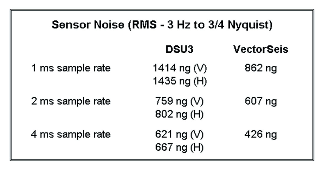
A primary objective of the VectorSeis design is the reduction of sensor noise and mitigating the impact of noise is certainly desirable. However, the strength and statistical nature of this noise needs to be put in perspective. Total random noise, as measured on spread noise tests in the field, includes both environmental and sensor noise. It is typically an order of magnitude larger than sensor noise. Even in the most tranquil of environments total random noise exceeds sensor noise by a factor of 3. Both environmental and sensor noise can be treated as random ( although with perhaps different distribution functions) and attacked through conventional increases in data redundancy. The level of required redundancy should be judged far more by environmental noise than sensor noise.

Sensor Overdrive/Recovery

The most noticeable differences in data acquired using the two sensors are typically best observed at the prestack stage and relate to differing overdrive levels and overdrive behavior of the two MEMS sensors. Overdrive level refers to the level at which a sensor reaches full scale and overdrive behavior describes how quickly the sensor recovers from being overdriven. Since both MEMS sensors utilize accelerometers, it is natural to describe the overdrive levels in comparison to the Earth gravity acceleration, G, which is 9.81 m/s2. The overdrive levels typically observed are 0.459G on DSU3 data and 0.225G on VectorSeis data.

Figure 8 provides data samples from a Canadian test and demonstrates the expected comparative overdrive behavior for the two sensors. The data suggest rather lengthy recovery times following overscaling for the VectorSeis sensor.

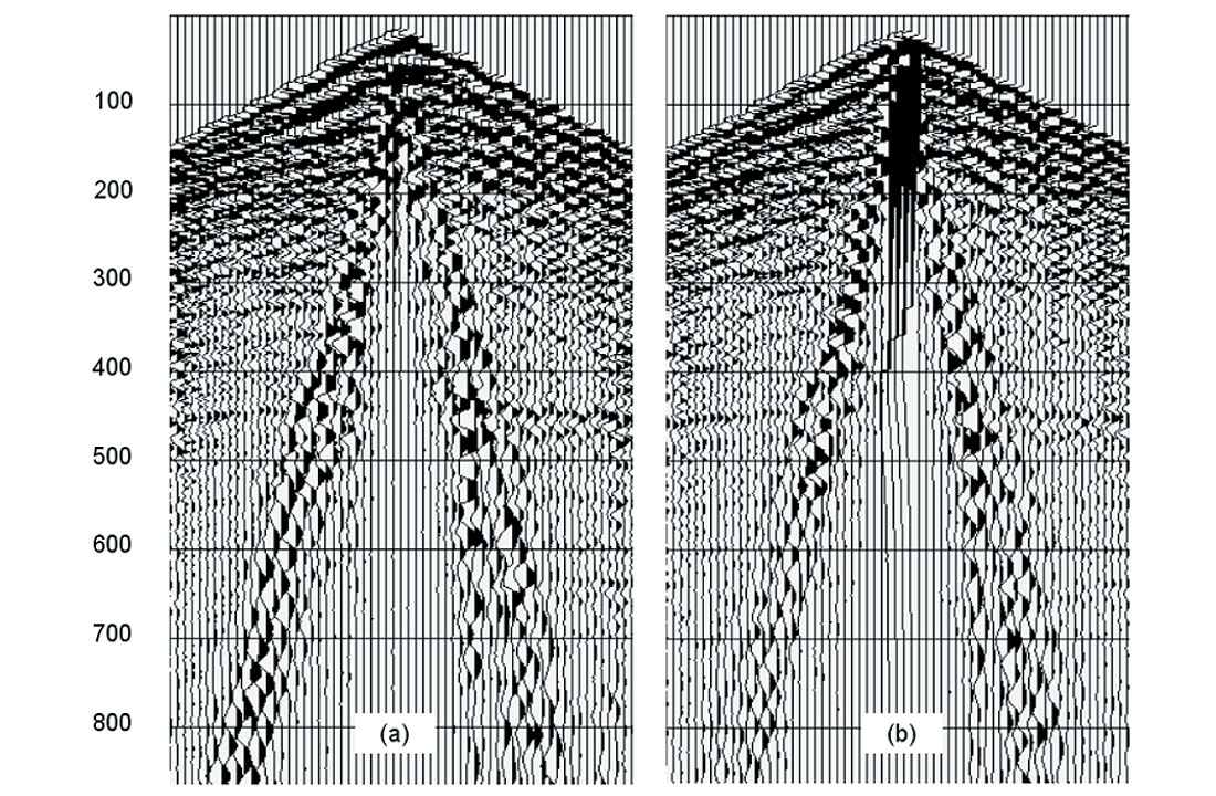
Sensor overdrive is not a new phenomenon but long recovery times are. Might it have more significance for converted-wave recording? Perhaps. In the shallow heavy oil play of NE Alberta, Canada, there is a rather significant loss of data in the first 250 – 500 ms of several near traces for each shot. Since converted-wave data typically have lower signal-to noise than corresponding compressional-wave data, preserving every possible trace is desirable. The user can best judge the importance of this issue as a function of specific parameters such as target depth and available fold.

Sensor Testability

Sensor testing has long been an industry standard and considered an essential practice in validating system integrity particularly as equipment ages. There are a number of reasons for a MEMS device, as for a geophone, to shift out of specification over time while remaining functional. These can relate to, for example, long term vacuum leakage of the cavity, drift of bonding contacts with time and temperature and spring damage resulting from substantial sensor shock. In sum, sensor degradation is to be expected and a performance watch necessary.

The Sercel DSU3 sensor has a built-in generator that excites each sensor element, allowing dynamic quality control of the sensor. The measurements from the excitation are compared to a table of theoretical values to validate sensor performance. Available tests are listed in Table 2 and compared among the transducers discussed in this paper.

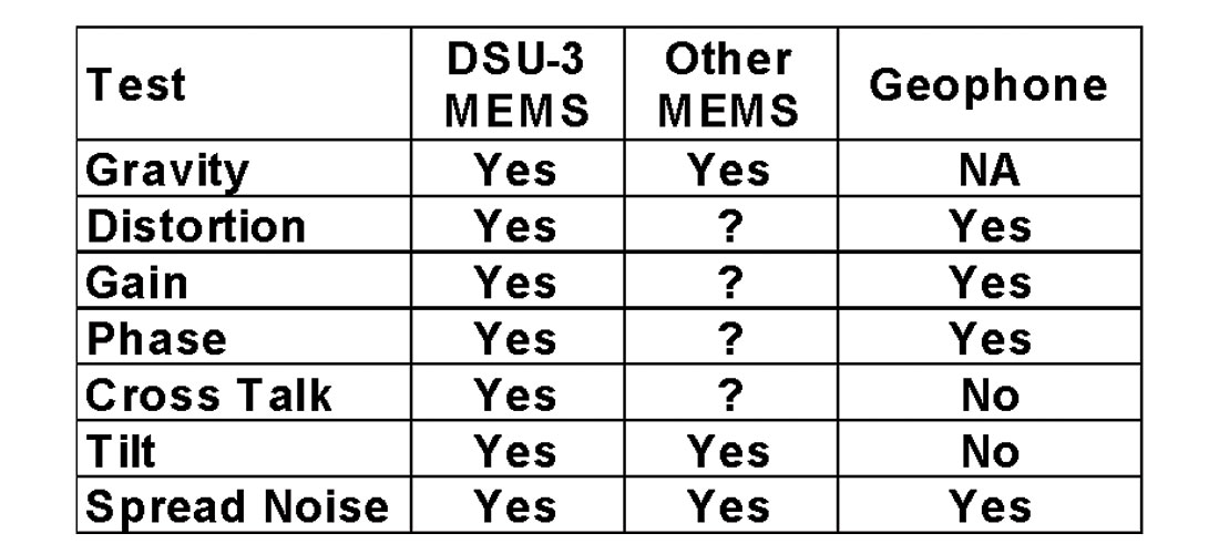
DSU3 sensor testing to date by Veritas on quite new equipment has demonstrated less than a 1% failure rate for the suite of distortion, gain, phase and cross-talk tests. Whenever a failure occurs, appropriate action is taken to ensure that specifications are met. With single sensor recording for multicomponent acquisition it is essential that every sensor perform as expected and it seems prudent to test field equipment as in the past.

Summary

Although designs among MEMS sensors vary, there should be no concern about loss of dynamic range with typically observed sensor tilt. Legitimate concern, however, exists for the use of systems with elevated power requirements and without test capability. Power consumption must be managed at every opportunity to promote efficient recording of large channel counts. Single sensor recording requires attention to the performance of every sensor deployed and to reducing data losses such as those due to overscaling.