AVO and Lamé Constants for Rock Parameterization and Fluid Detection

Introduction

For more than 3 decades, industry has known that shear seismic waves (S-waves) contain different rock information than do our standard compressional seismic waves (P-waves). Periodically, efforts to record S-waves, even on the seabed, have attracted industry attention with increasing success. Separate efforts to analyse conventional P-waves for the S-wave information contained or missing within them, have had more success and popularity as a function of significantly lower recording cost and relatively simpler analysis. These methods termed AVO (amplitude versus offset) are a logical and quantifiable petrophysical extension into pre-stack seismic data from the confusing and simplistic interpretation of stacked amplitudes. Since the mid 90’s new AVO inversion methods have been gradually succeeding in the Western Canadian Sedimentary Basin (WCSB), most notably in the exploration and development of gas pools within both clastic and carbonate plays. The improved approach described in this paper, combines conventional seismic AVO with petrophysical log analysis through the understanding of the fundamental Lamé parameters of rigidity Mu (μ) and incompressibility Lambda (λ). These parameters form a common theme between the varied aspects of AVO and log analyses considered and necessitate the use of some equations that are relatively simple to follow and hopefully reveal a deeper insight into the connection between rock physics and quantitative AVO.

Standard industry AVO methods exploit anomalous variations between seismic compressional wave velocity (Vp) or impedance (Ip) and shear wave velocity (Vs) or impedance (Is), to indicate changes primarily in pore fluid, as well as lithologic properties (Gassmann 1951, Pickett 1963, Tatham 1982, Castagna 1993a). Other methods using AVO measurements derive Poisson’s ratio (Ostrander 1984, Shuey 1985, Verm & Hilterman 1995) or P and S reflectivities, i.e. impedance contrasts (Gidlow et al.1992, Fatti et al.1994, Wallace & Young 1996). The emphasis on seismic velocity and density arises from the Knott-Zoeppritz equations for continuity of displacement (u) and stress (σ) across interfaces between different lithologies for a propagating seismic wave. Displacement and stress are usually derived from a plane wave solution of the acoustic wave equation; u = Ae^iω(t-x/V). However the underlying physics in the wave equation; d²u/dx² = ρ/M (d²u/dt²) does not involve seismic velocities, but instead the ratio of density (ρ) to modulus (M).

This paper will show that understanding velocity or impedance measurements in Lamé parameter terms of rigidity μ and incompressibility λ, offers new insight into the rock property factor ρ/M that governs wave propagation. In what follows, λ is considered to be pure incompressibility and not the bulk modulus , as λ is the only modulus involved in both the hydrostatic stress-strain relationship and acoustic wave propagation for a fluid (i.e. where rigidity μ vanishes). In addition to these Lamé parameters λ and μ, two new attributes LambdaRho (λρ) and MuRho (μρ) (Lamé impedances) are obtained from AVO by using moduli and density relationships to impedance. An improved identification of reservoir zones is possible by the enhanced sensitivity to pore fluids from pure incompressibility λ or λρ. Furthermore a better understanding of lithologic variations independent of fluid effects, such as sand/shale ratio can be obtained by analysing fundamental changes in rigidity μ, incompressibility λ, and density ρ parameters as opposed to a mixture of parameters within seismic velocities or impedances.

Theory and methods

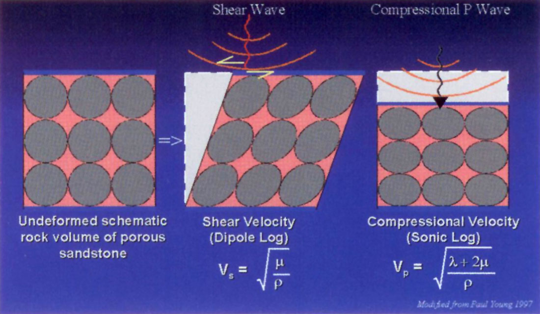
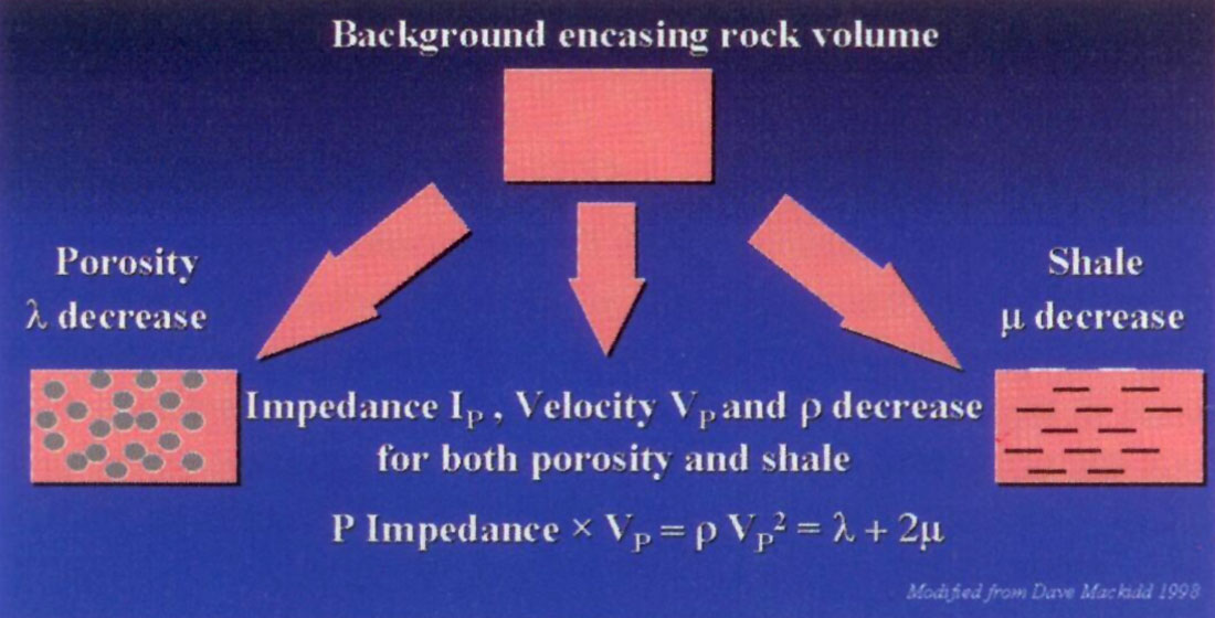
The dependence of seismic wave propagation on moduli is not obvious in standard AVO methods that rely on intercept and offset gradient, P-wave and S-wave reflectivity (Rp, Rs) or velocities Vp/Vs and Poisson ratio variations. Some authors point out the need for a more physical insight afforded by rigidity μ (Wright 1984, Thomsen 1990, Castagna et al. 1993b). Castagna also indicates that the link between velocity and rock properties for pore fluid detection is through the bulk modulus κ that is embedded in Vp. However, as λ relates uniaxial and lateral strain to uniaxial stress, it is primarily a longitudinal measure and hence orthogonal (i.e. independent) to μ, a quantity that relates a shearing stress to strain. This is not the case for since it implicitly relates to a measure of shear strain due to the volume’s change in shape resulting from triaxial or hydrostatic stress. This confusion can be seen in the following relationships; Vp² = (λ + 2μ)/ρ = (κ + (4/3)μ)/ρ (where κ = λ + (2/3)μ) and Vs² = μ/ρ and is further developed in the sections explaining moduli. Figures 1 and 2 show how the mixed parameters within velocity (Vp) for the compressional wave experiment result in an ambiguity in discriminating porous sand from shale. The equivalent and simpler shear experiment measures shear velocity (Vs) that is proportional to rigidity μ and thereby has less ambiguity discriminating between sand and shale. However a measure of rigidity alone is unable to provide a direct estimate of fluids within the sand pore volume.

Hooke’s Law explained in Lamé moduli terms

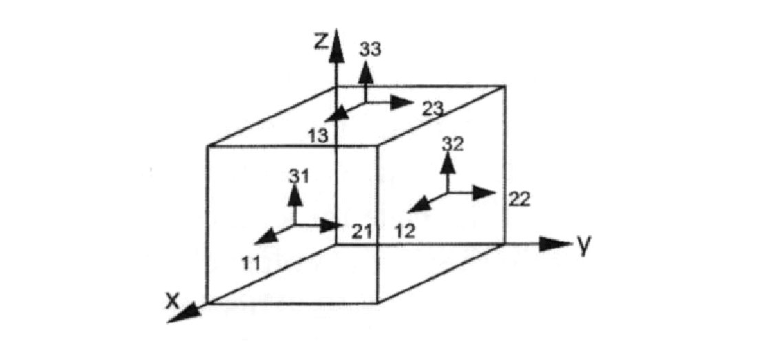
Hooke’s law relates the rank 2 tensors of stress (σ) to strain (e) with indices ‘j’ and ‘l’ being face normals and ‘i’ and ‘k’ the directions of stress or strain in a Cartesian system of x, y and z. The particle displacement vector u also has indices ‘j’ and ‘l’ denoting x, y or z directions.

Hooke’s law; σ_ij = c_ijkle_kl

where strain

as represented in derivative indical notation (notation as used in appendix for wave equations)

Stiffnesses c_ijkl quantify the stress to strain ratio and are rank 4 tensors (i.e. relating the rank 2 stress σ_ij to strain e_kl tensors) given as;

c_ijkl = λδ_ijδ_kl + μδ_ikδ_jl + μδ_ilδ_jk

This expression contains the Lamé parameters or moduli of a single incompressibility, Lambda (λ) and two rigidity, Mu (μ) terms. These Lamé moduli are combined for specific directions of stress to strain tensor relationships, as constrained by the Kronecker delta function rules. For the λ term these constraints are δ_ij requiring that i = j and likewise δ_kl requiring that k = l. So we can see that as the stress and strain face normals and directions are in the same x, y or z direction, then this λ modulus relates to longitudinal or compressional quantities. However the μ terms are not so simple. As the two terms have the requirements of δ_ik δ_jl and δ_il δ_jk, so strain indices k, l are replaced by i, j. This means that the stress and strain indices have the same i and j directions and so these μ rigidity moduli appear in Hooke’s law relating compressional stress to strain i.e. i = j. This can be seen in the derivation for axial or compressional stress by substituting the expression for c_ijkl in Lamé moduli into Hooke’s law;

σ_ij = c_ijkle_kl = (λδ_ijδ_kl + μδ_ikδ_jl + μδ_ilδ_jk)e_kl

where δ_ijδ_kl ⇒i = j, k = l ⇒ λδ_ijδ_kle_kl ⇒ λδ_ijek_k

for the first μ term δ_ikδ_jl ⇒ i = k, j = l, with the second μ term δ_ilδ_jk ⇒ i = l, j = k
⇒ (μδ_ikδ_jl + μδ_ilδ_jk)e_kl ⇒ μe_ij + μe_ji = 2μe_ij

⇒ σ_ij = λδ_ije_kk + 2μe_ij where for axial stress i = j

⇒ σ_ii = λje_kk + 2μe_ii ⇒ in the x direction σ_xx = (λ + 2μ)e_xx + λe_yy + λe_zz

This confusing result shows that the rigidity modulus μ is involved in the stress-strain relationship for axial compression. A physical explanation to better understand this is that a compressional stress that alters the volume of a body must also change the body’s shape thereby invoking a resistance as a function of both the incompressibility modulus λ, as well as the rigidity modulus μ of the body’s material.

By contrast the pure shear or rotational stress-strain relationship is clearly a function of rigidity μ only i.e. from the change in the body’s shape alone. This is seen below by substituting the expression for c_ijkl in Lamé moduli into Hooke’s law to give;

σ_ij = c_ijkle_kl = (λδ_ijδ_kl + μδ_ikδ_jl + μδ_ilδ_jk)e_kl

where for shearing stress, strains i ≠ j, k ≠ l,⇒ λ_ijδ_kle_kl = 0

and the first μ term δ_ikδ_jl⇒ i = k, j = 1, with the second μ term δ_ilδj_k

⇒ i = l, j = k

⇒ (μδ_ikδ_jl + μδ_ilδ_jk)e_kl⇒ μe_ij + μe_ji = 2μe

⇒ σ_ij = 2μe_ij where for shear stress in the z direction on the “x normal” face

Defining seismic impedance and the relationship of modulus, density and propagation velocity from the wave equation and its plane wave solution

Seismic impedance is a fundamental quantity forming the basis for all reflection methods. However by being the product of propagation velocity and density, impedance is not an obvious quantity for the average practising geophysicist, unlike propagation velocity and hence arrival times. As AVO attribute analysis involves extracting Rp and Rs reflectivities or impedance contrasts and as the new Lamé impedances λρ and μρ stem from impedance inversion, so the following is a derivation of impedance and the relationship of modulus to velocity, from the wave equation.

Starting with the 1D acoustic wave equation;

(where particle velocity with particle displacement u = Ae^iω(t–x/v)

as a plane wave solution of the wave equation and σ is stress with V as propagation velocity)

Integrate both sides with respect to distance x;

next substituting

gives the definition of impedance I (I = ρV) as being the negative ratio of stress to particle velocity (Aki & Richards 1980, p137).

Also as pressure is defined as P = – σ so P = ρVν.

Continuing with this result the original wave equation may be written in terms of stress as;

So the wave equation can be simply stated as: “Propagation velocity V is equal to the negative ratio of the time to space derivatives of stress”.

Finally rewriting σ = – ρVν in terms of displacement where M is the medium’s modulus and using Hooke’s law gives;

Integrating both sides with respect to x gives;

replacing u = Ae^iω(t–x/v)

leading to the expression relating modulus, density and propagation velocity as M = ρV².

One of the consequences of the relationship of stress to the product of particle velocity and impedance, is that for the same initiating stress or pressure a seismic wave will have a lower particle velocity in a high impedance material than a low impedance material. As the low impedance material particle must travel further per frequency cycle (i.e. faster) than the high impedance material particle, so it will suffer more energy loss through frictional forces. This gives rise to the common observation that sound of seismic waves suffer less high frequency attenuation in high impedance materials such as steel or water when compared to low impedance material such as wood or air. Further insight through an understanding of the Lamé parameters in relationships involving the elastic wave equation and anisotropy, are given in the appendices.

Understanding common moduli and moduli ratios in Lamé terms.

As a consequence of combining the Lamé constants of rigidity μ and incompressibility λ in the stress-strain relationship for a body, they form the basis for more familiar moduli definitions. These are dependent on the form of the body and the nature of the stress i.e. bound insitu material (rock in the subsurface), an unbound bar (core) or bulk triaxial measurements (fluids under compression). Useful insight into common moduli and moduli ratio definitions can be obtained by conversion to basic Lamé terms.

1. Compressional P-wave modulus; bound uniaxial compression M = λ + 2μ. This is the modulus involved in P-wave propagation in the Earth for both surface seismic and sonic logging.
2. Young’s modulus or unbound uniaxial compression; Y = λ(1-2σ) + 2μ or Y = M - 2λσ. The unbound nature of this measurement (e.g. a core) reduces the stiffness of the body as seen by the last equality where bound modulus M > Y by a factor of 2λ times Poisson’s ratio. The factor of two is a result of λ acting in both unbound lateral directions.
3. Bulk modulus; κ= λ + (2/3)μ or = M - (4/3)μ where the reduced unbound rigidity of the bulk modulus compared to the bound M modulus can be seen from M > by a rigidity factor of (4/3)μ. The bulk modulus contains a rigidity term (2/3)μ as a consequence of a triaxial stress changing not just the volume of a body (i.e. a compressional resistance as a function of incompressibility λ), but also its shape (i.e. a shearing resistance as a function of rigidity μ). This is my objection to calling the bulk modulus incompressibility (in favour of Lambda) as contains an element of rigidity.
   
   Alternatively the bulk modulus can also be seen as a “triaxial Young’s modulus” from 3 = Y/(1-2σ).
4. Poisson’s ratio; σ = λ /(2λ + 2μ) and Vp/Vs ratio =

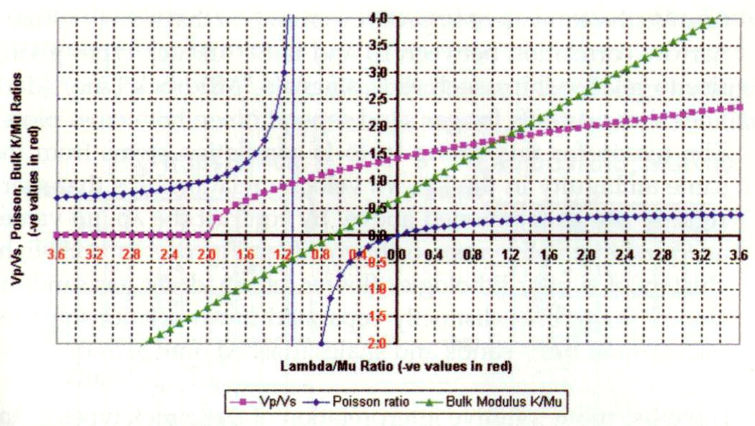
As the various definitions for moduli and moduli ratios contain mixtures of λ and μ, so there are some inconsistencies in considering negative λ‘s with positive μ‘s for sedimentary rocks. For example the bulk modulus is still positive for negative λ‘s, until -λ = (2/3)μ beyond which it is negative. However Poisson’s ratio is negative for negative λ‘s until at -λ = μ, Poisson’s ratio is infinite and discontinuous, returning to being positive for -λ > μ. These impossible and non-linear variations of bulk modulus and Poisson ratio with the fundamentally unambiguous λ/μ ratio are shown in the graph below (figure 3). Further discussion and potential explanation of the confusion is given in the following section on improved sensitivity using Lamé attributes.

Poisson’s ratio, σ = λ/(2λ+2μ) or 2σ/(1-2σ) = λ/μ and (Vp/Vs)² = (λ/μ)+2, as given above are close to the most sensitive moduli ratio of λ/μ. Unfortunately the non-linear complexity of σ in Lamé terms (Thomsen 1990) and the constant 2 in (Vp/Vs)², reduce the full impact of the relative λ/μ ratio change between lithologies or fluids within lithologies. This can be seen for positive values in figure 3, as a reduction below the 1:1 line in the slopes or relative ranges of Poisson’s, Vp/Vs and bulk modulus/Mu ratios versus the larger λ/μ ratio range. The relationship λ/μ = 2σ/(1-2σ) is interesting as it shows that for a change in Poisson ratio, the numerator increases as twice the σ change while the denominator is reduced by 1-2σ thereby enhancing the λ/μ change to a maximal asymptotic approach for σ = 0.5 where λ/μ is infinite.

Lamé constants used in improved AVO attribute sensitivity for fluid/lithology discrimination.

The basic proposal in this paper is to use moduli/density relationships to velocities V or impedances I, given as:

Ip² = (Vp. ρ)² = (λ + 2μ) ρ and Is² = (Vs. ρ)² =μρ.

These relationships enable extraction of the orthogonal Lamé parameters λ and μ from logs with measured density ρ, or λρ and μρ from seismic without density. The simple derivations are:

λ = Vp².ρ – 2Vs².ρ, μ = Vs².ρ, and λρ = Ip² – 2 Is², μρ = Is².

Incompressibility λ is not directly measurable in rocks unlike rigidity μ, but the extraction can be seen as a form of stripping off the μ sensitive rock matrix to reveal the most sensitive pore fluid indicator λ.

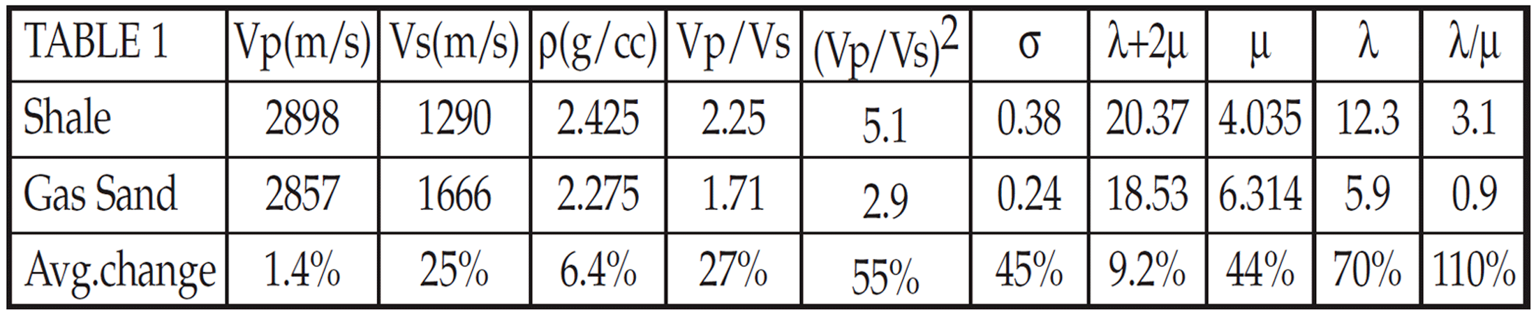
Table 1 shows the justification and power of the method in petrophysical analysis. Actual Vp, Vs and ρ values from a shallow gas well (not in the study area discussed later) have been combined to give various rock property values and average % change i.e. contrast at the interface for detectability. The unusual behaviour of a very limited Vp change (1.4%) compared to Vs (25%) for this thick, good quality gas sand zone requires some explanation, as most standard measurements concentrate on this non-responsive Vp change. The answer lies in comparing the last four columns, where it is apparent that because of Vp’s dependence on both λ and μ, the effect of decreasing λ as a direct response of the gas porosity is almost completely offset by an increase in μ in going from capping shale to gas sand. However by breaking out λ from Vp and combing it into a λ/μ ratio, average changes of 70% for λ and 110% for λ/μ are by far the most sensitive to the variation in rock properties between shale and gas sand. The best conventional measurements from Poisson’s ratio (σ) of 45% and (Vp/Vs)² of 55% are far less sensitive.

Distinguishing porous sands within varied channel facies can be difficult to impossible using common AVO attributes such as Vp/Vs and Poisson ratio as seen in table 2 below (highlighted in yellow) .

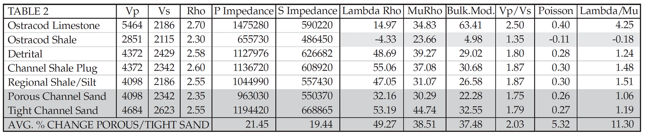
Table 2 compares log derived values for typical Glauconite incised valley and regional Ostracod facies in the WCSB. The improved discrimination between highlighted porous versus tight sand shown by impedance attributes of λρ (49%) and μρ (39%) is significant by comparison to Poisson’s ratio of only 5% and (Vp/Vs) of 2%. Note that P impedance has a reasonable 21.5% change between the same channel sand facies and this is routinely exploited by standard interpretation of stacked seismic amplitudes. However P impedance alone shows a small 13.4% discrimination between porous channel sand and channel shale plug, whereas λρ has a 38% discrimination. Following the moduli comparisons in the previous section, further confusion between positive and negative moduli and ratios can be seen in table 2, highlighted in green for the Ostracod shale. The log measurements give a negative Lambda and Poisson ratio but positive bulk modulus. Why is this so inconsistent? On the one hand Lambda and Poisson’s ratio suggest an impossible material where a compressive longitudinal stress results in longitudinal and lateral contraction in strain. By contrast there is nothing too unusual for this shale with positive bulk (and Young’s) modulus, suggesting that a normal triaxially compressive stress would result in a volumetric contraction. The standard argument for the positive bulk modulus is that for negative Lambda a material offers resistance to triaxial compression as a function of its rigidity Mu, but would still have a permissible negative Poisson ratio causing a lateral contraction for uniaxial longitudinal compression in an unbound state. The implication is to believe the moduli over the ratio, either the positive bulk or Young’s moduli. However by considering Lambda as a real and fundamental modulus for incompressibility, these conflicting values for both bulk and Young’s moduli must be just mathematical inconsistencies as a consequence of the elastic experiment used to obtain them resulting in mixed and confusing combinations of Lambda and Mu.

To emphasise this point, if one considers the hydrostatic case for a fluid where the bulk modulus is most applicable (Grant and West 1965 “Interpretation Theory in Applied Geophysics” p25-26) with no rigidity (μ = 0), then the argument for a negative Lambda which would give a negative bulk modulus, and positive Poisson’s ratio (σ = 0.5) would be considered impossible; this example has none of the confusion associated with a solid (Feynman 1963 “Lectures on Physics” Vol 2, p38-3). Therefore Lambda is a better fundamental measure of a material’s incompressibility and the results for the Ostracod shale in table 2, are more a function of erroneously low Vp sonic log measurements in this shale.

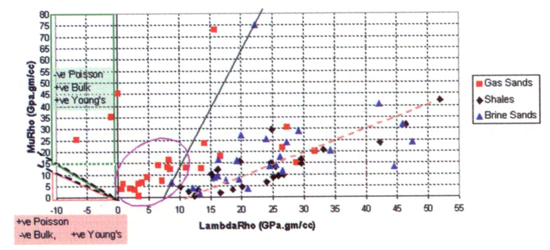
Continuing this log-based analysis of various moduli and AVO attribute sensitivity, the following graphed figures 4 and 5 compare Castagna and Smith’s (1994) published world-wide logs plotted as P impedance versus S impedance compared to the equivalent LambdaRho versus MuRho cross-plot.

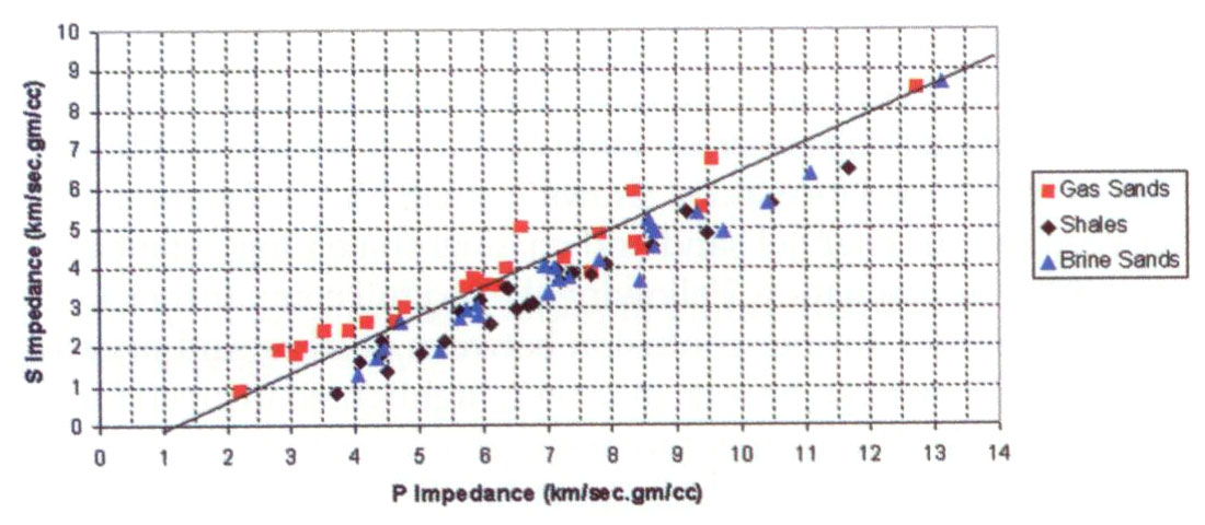
A number of interesting observations can be made by comparing the cross-plots:

1. There is clearly a better separation of the gas sands from brine sands and shales in the λρ, μρ cross-plot as all the space is now available for lithology and fluid characterisation. This is not the case for the equivalent impedance cross-plot that shows a strong narrow correlation between Ip and Is for all rock types giving rise to relationships such as Castagna’s “Mudrock Line” (dark lines show cut-offs for gas sand separation on both cross-plots). The reason for this strong Ip to Is correlation stems from the same ambiguity in the Vp, Vs velocity relationships that share rigidity Mu as mentioned above. By contrast the λρ, μρ values are fundamentally more orthogonal giving rise to both tight clusters of similar lithologies (lower left quadrant gas sands as circled) as well as distinctly separated linear relationships for background brine sands and shales (dashed orange line).
2. There is a more intuitive interpretation of these rock types in λρ, μρ cross-plot space, where the circled low μρ gas sands are most likely younger, less consolidated sands than the three gas sand values that appear well separated in the upper left quadrant (high μρ range). However, once again these three isolated points have either zero or negative Lambdas and Poisson ratios, but positive bulk and Young’s moduli. So the values could be used for modelling by Gassmann fluid substitution without any thought to the possibility that the logs are in error. Even further confusion would arise if any of the low μρ gas sands were to fall in the negative Lambda region shown by the lower left orange triangle as then Young’s modulus and Poisson’s ratio would be positive and believable while the bulk modulus and Lambda would be negative. My conclusion from the λρ, μρ cross-plot mapping of the confusing positive to negative non-linear behaviour for bulk, Young’s moduli and Poisson’s ratio within the clearly consistent negative Lambda region, is that Lambda alone represents the material’s true incompressibility and the other parameters disguise measurement errors.

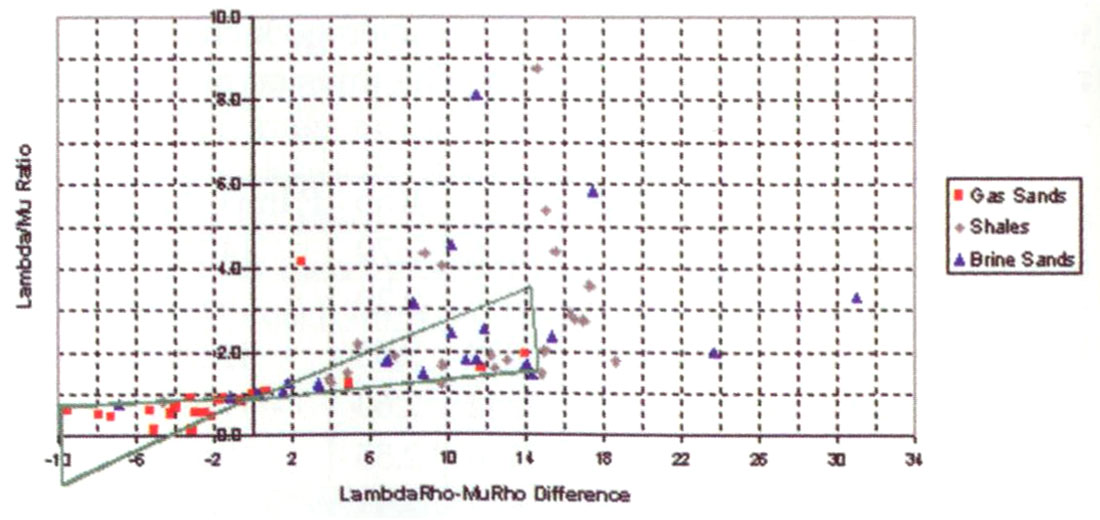
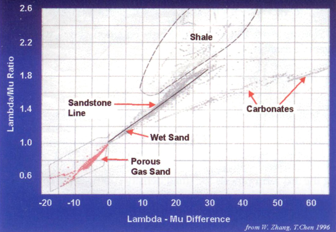
Following this cross-plot analysis for the same log data set, figure 6 below shows an interesting cross-plot (derived by T. Chen, W. Zhang and myself) of the λ/μ ratio versus the λρ-μρ difference. The two green triangles that meet at the (1,0) ‘origin’ show that the gas sands align within the lower left triangle while the brine sands tend to align in the upper right triangle. This alignment into lithologic “sandstone” lines with linearly varying fluid properties is explained in the next section on interpretation templating of Lamé attributes from log analysis from the Western Canadian Sedimentary Basin.

Log analysis motivation and interpretation template for Lamé parameters λ, μ, λρ and μρ.

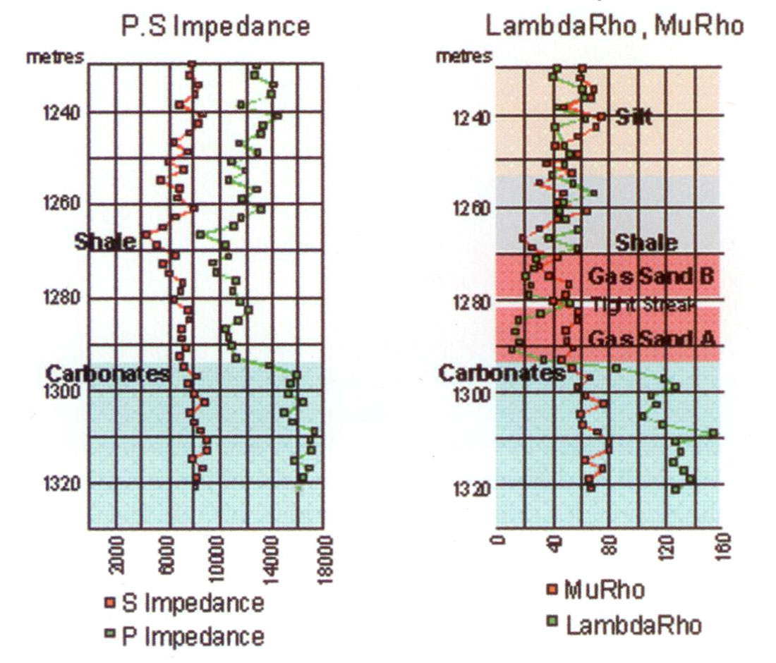
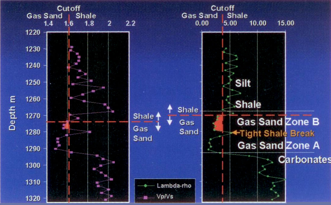
Figures 7a and 7b show a gas well sonic and dipole logs in depth where a conventional impedance Ip versus Is analysis has limitations in clearly discriminating between all the various lithologies and gas sand zones (e.g. only gas zone Ais discernible from a background cut-off on the Vp/Vs curve in fig.7b). Because Ip and Is share both rigidity and density, the log curves in figure 7a tend to track each other and never crossover, with only the lowest impedance shale or highest impedance carbonate zones being clearly distinguishable. By contrast the λρ and μρ curves (fig.7a) have similar value ranges and they do crossover with λρ < μρ for gas zones. Beyond this crossover there is the benefit of immediate diagnostic information for gas zone A showing a better poro-perm than zone B due to the larger curve separation in zone A. Conversely the λρ > μρ crossover is an excellent indicator of thin, tight shale breaks as seen separating gas zone A from B, as well as the capping shale above gas zone B. Figure 7b, compares just the λρ with Vp/Vs log tracks for gas sand detection sensitivity. Cut-offs for both log tracks were chosen based on the lowest values for the overlying background shales and silts. The upper gas zone B is clearly distinguished on λρ, unlike Vp/Vs, with λρ in agreement with the correct gamma log depth for the gas sand.

In general, seismic AVO analysis involves some form of crossplotting such as reflectivity-based intercept/pseudo-Poisson ratio (Verm and Hilterman 1995) or intercept/gradient (Castagna and Swan 1997). Further log analysis for AVO interpretation has lead to a “fluid factor” separation (Smith & Gidlow 1987) from cross-plots of reflectivity Rp versus Rs or Ip versus Is. Figure 8 compares the Ip, Is to λρ, μρ cross-plots for the gas sand log tracks in figure 7, with λρ, μρ showing a significant advantage in isolating both lithologic properties, e.g. sand, shale, and carbonate facies, as well as the gas zone’s fluid effects. The Ip, Is points in figure 8 cluster in a tight linear relationship (i.e. Castagna’s “Mudrock Line”) with shale having the lowest values on both axes. By contrast the lowest λρ values in the λρ, μρ cross-plot discriminate the best gas sand zone A, along with higher μρ values than the background shales. Simply put, for the Ip, Is cross-plot all rock types plot to the upper right direction from the lowest shale values. Conversely for the λρ, μρ cross-plot, the anomalous gas sands plot in the upper left hand quadrant from the lowest μρ shales, while other more competent or tight lithologies (silts, cemented sands) plot in the opposed, upper right quadrant relative to the shales. As mentioned before, the reason for the separation improvement in the λρ, μρ cross-plot compared to Ip, Is, is that the λρ versus μρ axes are orthogonal with regard to Lamé parameters or moduli, unlike Ip versus Is, thereby making the cross-plot more discriminating.

λρ, μρ showing a significant advantage in isolating both lithologic properties, e.g. sand, shale, and carbonate facies, as well as the gas zone’s fluid effects. The Ip, Is points in figure 8 cluster in a tight linear relationship (i.e. Castagna’s “Mudrock Line”) with shale having the lowest values on both axes. By contrast the lowest λρ values in the λρ, μρ cross-plot discriminate the best gas sand zone A, along with higher μρ values than the background shales. Simply put, for the Ip, Is cross-plot all rock types plot to the upper right direction from the lowest shale values. Conversely for the λρ, μρ cross-plot, the anomalous gas sands plot in the upper left hand quadrant from the lowest μρ shales, while other more competent or tight lithologies (silts, cemented sands) plot in the opposed, upper right quadrant relative to the shales. As mentioned before, the reason for the separation improvement in the λρ, μρ cross-plot compared to Ip, Is, is that the λρ versus μρ axes are orthogonal with regard to Lamé parameters or moduli, unlike Ip versus Is, thereby making the cross-plot more discriminating.

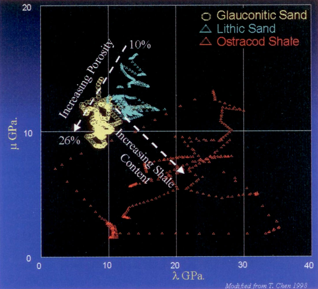
Continuing with this log-based template interpretation, figure 9 shows a λρ versus μρ cross-plot of logs for a Mannville gas sand interval with two very different sand porosities (Lithic and Glauconitic) as well as the background Ostracod shale. There is a clear clustered separation of the gas sands representing a difference in porosity as shown by the increasing porosity trend toward the origin. A sand/shale lithology change is seen to occur in the opposed direction normal to the porosity trend, thereby clearly isolating the Ostracod shale from varying sand porosities. These porosity and sand/shale trends would tend to be more confusingly aligned in the same direction on the equivalent impedance crossplot of Ip versus Is, as compared in figure 8 above.

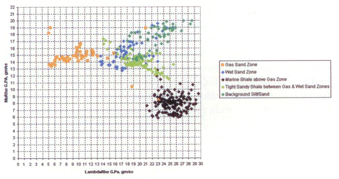
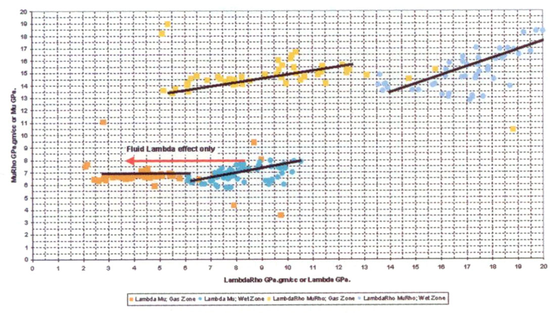
A more detailed interpretation template is shown in the following λρ versus μρ cross-plots in figures 10a and b. These logs for a shallow Viking sand interval will be used in a following section on a 3D seismic AVO and VSP case study. Figure 10a shows a diagnostic separation of lithologies with the marine shales in black (Base of Fish Scales overlying the Viking sand) clustering with the lowest μρ‘s and highest λρ‘s. The terrigenous shales that surround the porous sand zones and the background silt/tight sands show separate trends dependent on the relative sand/shale content versus porosity (compare to figure 9). By contrast the gas to wet sand separation is primarily a function of the horizontal decrease in Lambda as a fluid effect seen in both figures 10a and b. However figure 10b shows that a density effect can be discerned by comparing the upper (λρ versus μρ) to lower (λ versus μ) pair of gas versus wet sand clusters. The increased density trend slopes for the upper paired clusters (i.e. varying ρ on both axes) are not as obvious as the larger horizontal Lambda fluid effect in going from wet to gas sands, as shown by the red arrow.

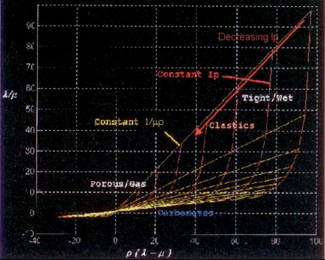
The final portion of this section on cross-plot template interpretation deals with the additional discrimination of fluid and lithology effects using the λ/μ ratio versus λρ-μρ difference cross-plot introduced in figure 6. The template shows that rocks of consistent lithology will tend to align as lines of constant μρ (actually 1/μρ) radiating through a ratio, difference “origin” of (1,0). The variation along these lines will be primarily driven by fluid or saturation effects (i.e. decreasing λρ toward and through the (1,0) origin), with porous gas sands trending to the lower left quadrant from the (1,0) “origin” (as in figure 6).

A proof (derived by D. Cooper 1997) of the constant lithology μρ lines can be shown as follows.

The slope of a line through the (1,0) “origin” of figure 11 for two points 1 and 2 on the line is given as

assume at least one point on the line (point 1 in the equation) is fixed at the (1,0) “origin” so at (1,0) λ = μ i.e λ / μ = 1 (∴ Vp/Vs = √3 ) and (λ – μ)ρ = 0, then the slope equation reduces to

making the slopes proportional to the reciprocal of μρ

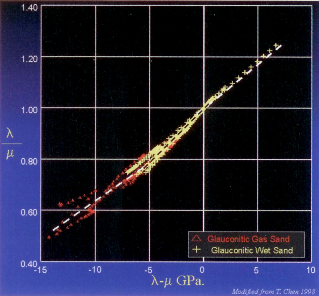
Figures 12a and b show the interpretation template for this λ/μ ratio versus λρ-μρ difference cross-plot for logs from a Glauconitic sand interval. The constant 1/μρ line termed a “sandstone line” shows varying gas to water saturations along its length, with the higher gas saturation through the (1,0) “origin” in the red area. A detail of this area is shown in figure 12b, where the gas zone is seen to be better isolated beyond the (0.8,-5) point rather than the (1,0) “origin”. The variation of slope with increasing gas saturation (black to white dotted lines) reveals an unexpected effect of the fluid on the rigidity of the sand.

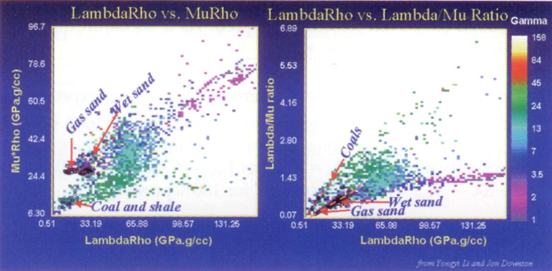
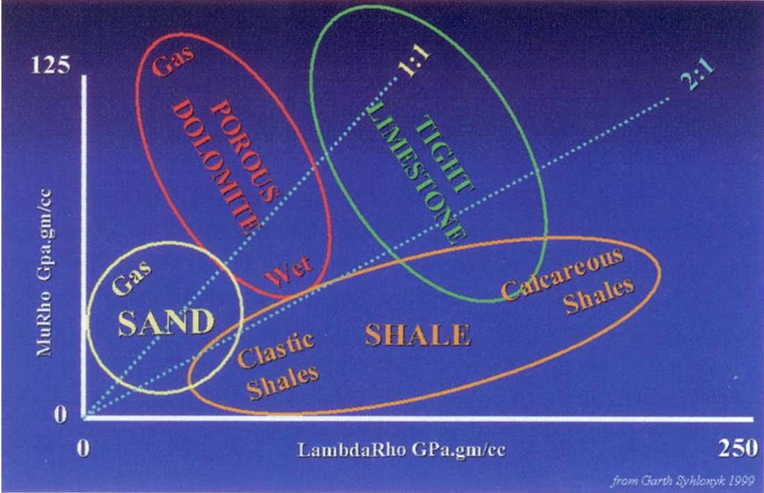
Further templates showing the relation between gas, wet sand and coals are seen in the pair of λρ versus μρ and λ/μ ratio versus λρ-μρ difference cross-plots of figure 13 from Y. Li and J. Downton. Afinal simple schematic compilation of these various lithologic and fluid/porosity effects is shown in figure 14 as a general guide.

Biot-Gassmann equation expressed in Lamé parameter terms.

The following common Biot (1956), Gassmann (1951) and Geertsma (1961) equations for fluid substitution and modelling are transformed into simpler Lamé parameter terms. This result is used as further motivation for the potential to directly extract meaningful pore fluid detection attributes such as Δλ and Δλρ, to be shown in the next section on AVO reflectivity equations and Lamé parameterisation.

Biot - Gassmann equation;

where Κ is Bulk modulus and “sat” is saturated rock with ϕ as porosity.

Lamé form of Biot - Gassmann equation assuming μ_dry = μ_sat ;

for detection of changes in fluids where Δλ = λ_sat – λ_dry and substituting ΔK = K_solid – K_dry

with a useful approximation based on K_solid >> λ_fluid and ϕ K_solid² >> λ_fluidΔK

The last approximate expression for Δλ as a fluid attribute shows that fluid detection is directly proportional to the fluid λ as well as the porosity effect in ΔΚ² and inversely proportional to the porosity scaled solid rock bulk modulus squared. As a check on this relationship consider the limits:

1. as porosity ϕ → 0 so ΔK → 0 therefore Δλ → 0 as expected as λ_sat = λ_dry
2. as porosity ϕ → 1 so ΔK = K_solid as K_dry → λ_dry = λ_air = 0 therefore Δλ → λ_sat = λ_fluid as expected for 100% porosity

Finally one prediction from this form of the Biot-Gassmann- Geertsma equation is that Δλ fluid detection is enhanced for rocks with lower bulk moduli (denominator) and higher porosities (numerator ΔΚ²) such as poorly consolidated sands, thereby confirming actual observation.

Angle dependent reflectivity equations and approximations for AVO seismic or VSP analysis

This section will compare two basic approaches for extracting AVO attributes, one for P-wave and pseudo-Poisson reflectivity, the other for P and S reflectivities (Rp(0°) and Rs(0°)) which can be inverted into λρ and μρ. Some AVO inversion schemes incorporate an explicit density term (Stewart et al. 1995, Smith 1996) to potentially extract moduli and density separately. However as the number of unknowns increase and exceed the measurable CMP gather quantities (intercept and gradient) so these more complex equations are less robust and the extracted values more ambiguous. This is especially true in the presence of noise where even two attributes such as Rp, Rs are in doubt (Cambois 2000).

A common starting point for AVO analysis is the tractably linearized 3 term approximation to the Knott-Zoeppritz equations given by Aki and Richards (1980) shown below with an explanation of assumptions. These form the starting point for yet further 2 term approximations used to extract Rp(0°) and Rs(0°) or pseudo- Poisson reflectivity. The basic linearized assumptions in the Aki and Richards approximation are small fractional velocity and density changes with 2nd order terms ignored and θp < 10 degrees of critical.

where: Vp, Vs velocities, ρ density, are averaged across an interface and angle θp (or just θ) is the average of incident and transmitted P-wave. ΔVp/Vp, ΔVs/Vs, Δρ/ρ are fractional changes in Vp, Vs and ρ across an interface and can be considered equivalent to ΔlnVp, ΔlnVs and Δlnρ.

The first common industry method considered is a P-P AVO extraction of zero angle Rp(0) and Rs(0) “seismic traces” through “weighted stacking” of CMP gather data (Gidlow et. al.1992, Fatti et. al.1994).

Starting from the Aki & Richards equation above with some algebraic manipulation gives;

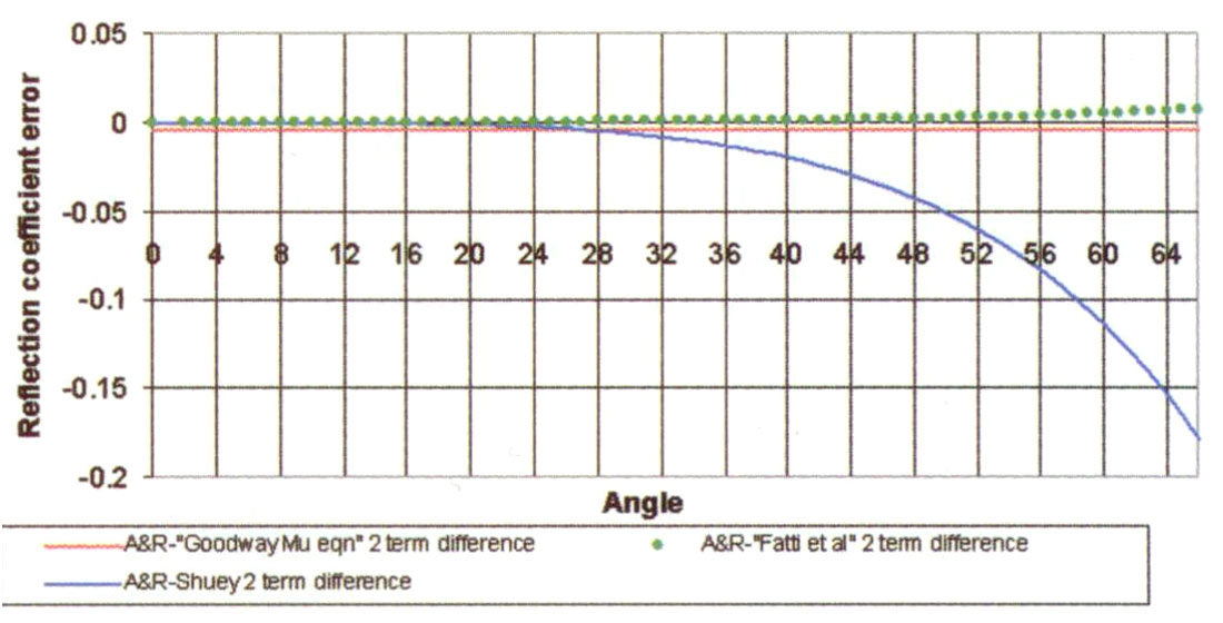
Equation (a) the “Geogain Equation” from Gidlow et. al., is solved in a least squares sense to extract Rp(0) and Rs(0) by assuming the 3rd term cancels for small density contrasts (Δρ/ρ), as well as for small angles i.e. tan²θp = sin²θp, and (Vs/Vp) = 1/2. If the density contrast is not small then this third “error” term can be significant at large angles and more importantly inconsistent for varying rock properties by being dependent on both angle and Vp/Vs ratio (see graph of angle dependent error below).

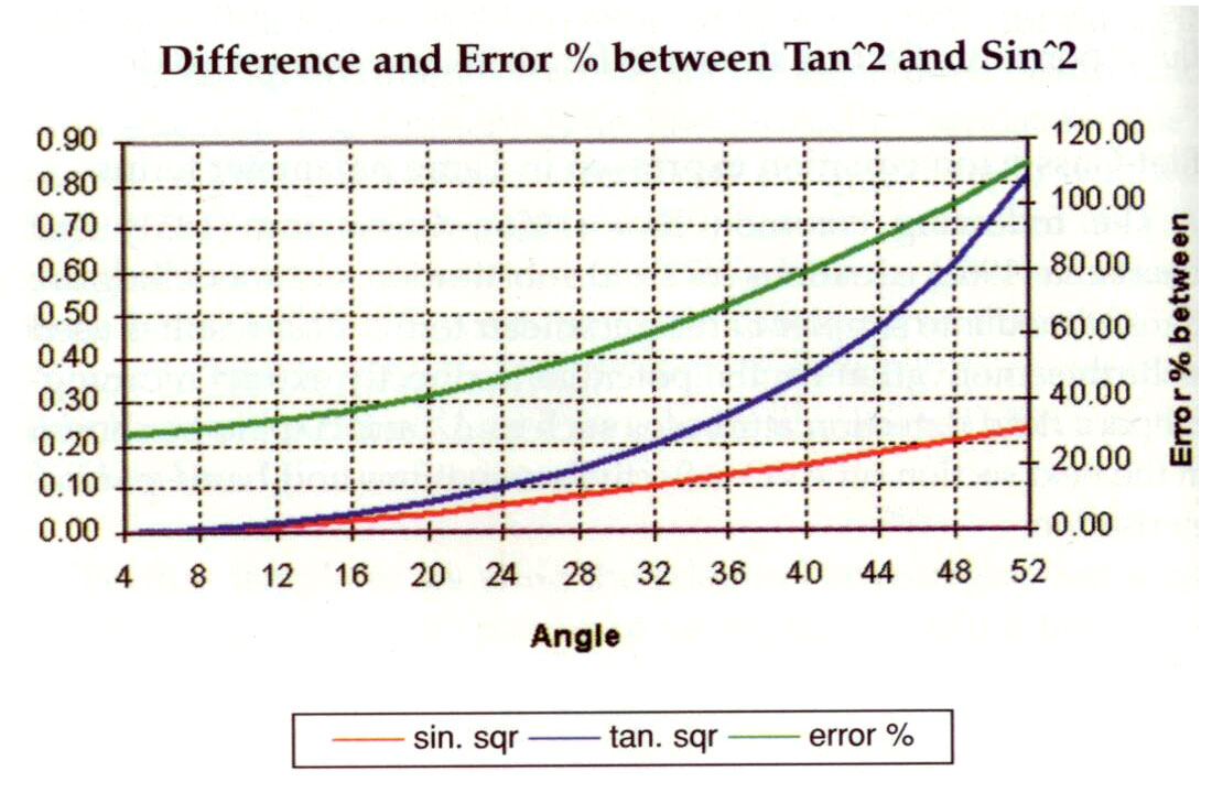
For Vp/Vs ratios < 2 the error between the approximate 2 term Fatti et. al. equation and the exact Aki & Richards 3 term curve is small and evenly distributed, but still angle dependent. However for ratios 2.5 or 3, this error increases with increasing angle and because the error term is strongly dependent on both angle and Vp/Vs ratio this restricts the useable range of angles.

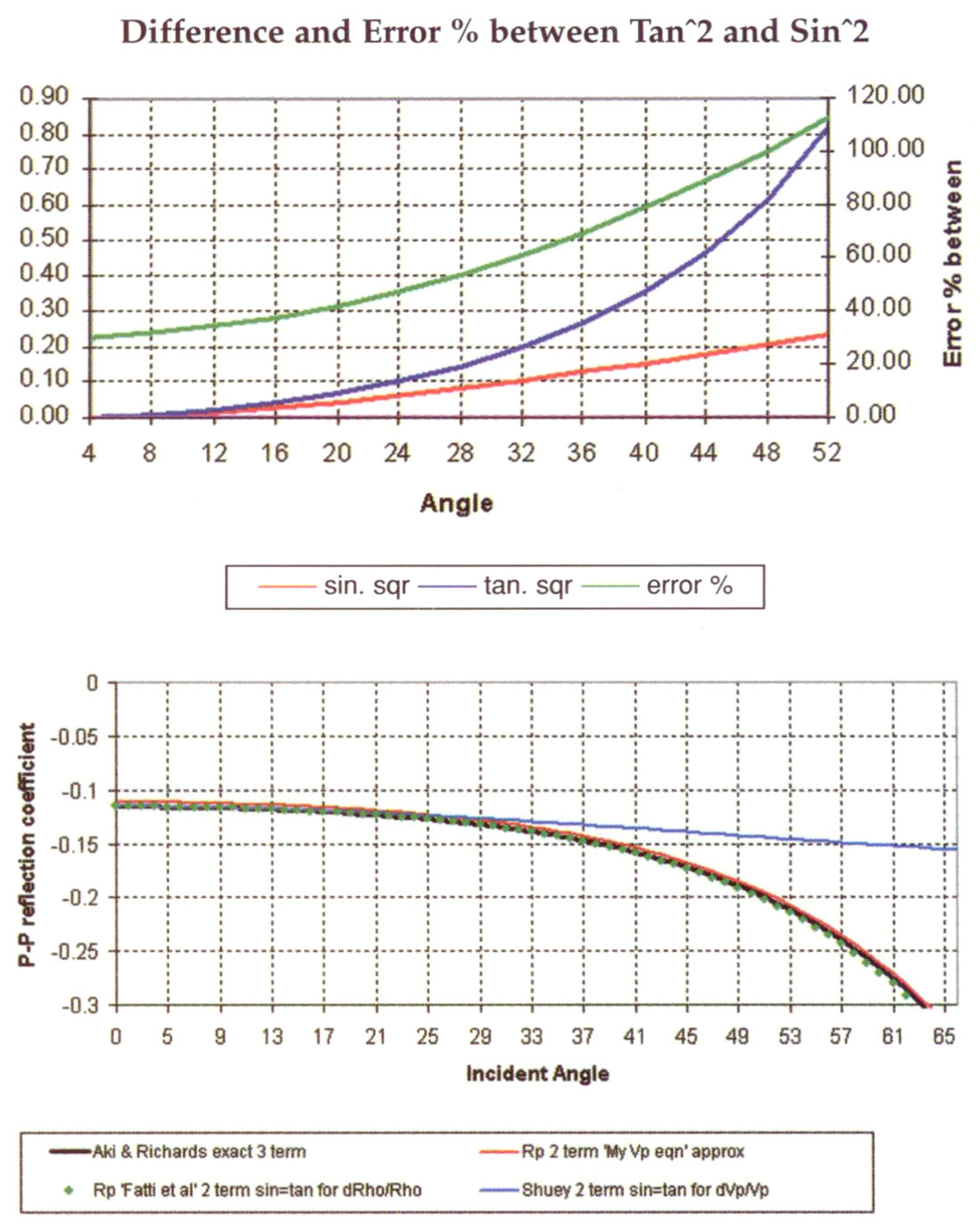
In practice, however, this equation is very useful and can be used to fairly large angles (see following AVO model curve comparisons figures 15a, b) as Δρ/ρ has the smallest variation compared to ΔVp/Vp and ΔVs/Vs, seen in Gardner’s (1974) relationship as Δρ/ρ ≈ (ΔVp/Vp)/4. If the angle range is restricted to a commonly quoted 30° due to the ignored error term, then the catch-22 problem is that the same large angle restriction reduces the separability of sin and tan curves involved in the remaining first two terms of equation (a). If this angle restriction can be reduced then more robust and independent estimates of ΔIp/Ip and ΔIs/Is are possible in theory.

The situation is much worse for the second industry method based on a 2 term approximation by Shuey (1984). The formulation is significantly more complex than the Fatti et. al. equation above and is just reproduced here for comparison.

The two term approximation for the Shuey equation (b) is to drop the 3rd term in (ΔVp/Vp) and this is where the infamous 30° angle restriction comes from, because dropping a term involving (ΔVp/Vp) is significantly worse than a Δρ/ρ term in the Fatti et. al. equation (a) (see Gardner’s relationship above).

However a different approximation with no angle dependent error can be obtained by substituting the following relationships into the original Aki & Richards equation;

Now the approximation in this equation (c) (Goodway 1997), is to drop the small zero offset term Δρ/2ρ (again from Gardner’s relationship Δρ/2ρ ≈ (ΔVp/Vp)/8). Note that this error is independent of angle unlike the Fatti et. al. or Shuey two term approximations (i.e. equations (a) and (b) without 3rd terms) and hence allows a more accurate fit to the exact Aki & Richards AVO curve at large angles, but has a “bulk” Δρ/2ρ scalar shift at all angles. These three 2 term approximations (equations a, b and c) are compared to the Aki and Richards three term equation as graphed against incident angle in figures 15a, and b.

Yet further interesting reformulations of the original Aki & Richards AVO equation can be obtained in terms of linear cos2θ only. A simplified AVO attribute extraction or analysis method using the FFT of equation (d) below in offset variable θ, gives very specific ΔVp/Vp and Δμ/μ scaled spectral notches/peaks as functions of cos2θ only;

and in Lamé moduli, density terms the Aki-Richards equation simplifies to:

Note there is no density influence on R(θ) at 45° i.e. R(θ) is just a function of moduli as a ratio that is almost Δ(Vp/Vs)²/(Vp/Vs)². This concurs with Hilterman’s work on far offset reflectivity (shown in an excellent book on AVO accompanying the SEG DISC 2001).

Next this Lamé parameterized equation can also be represented in cos 2θ terms:

that can be further simplified to;

or more usefully as a quadratic equation in terms of cos 2θ:

This final result shows a similar though more interesting insight, to equation (e) above. The insight here is that at θ = 45° cos2θ = 0 and so the reflectivity R(45) is just a scaled version of the change in the basic fluid indicator Δλ derived as follows (see motivating Lamé Biot-Gassmann equations in previous section).

Vp (product of averaged P impedance and velocity) and average Ip can be obtained following the basic definitions above for

Consider zero angle R (0) as a function of time τ :

⇒ 2 Σ R₀(τ) Δτ = ln(Ip) exponentiating gives ⇒ e^{2ΣR₀(τ)Δτ} = Ip

Average Vp or V (τ)_INT can be obtained from the standard Dix

V_RMS NMO relationship as;

(where T(τ) = -ΣΔτ and if V_RMS varies slowly or is constant in interval Δτ)

So as average

combining all these results gives;

Finally the Fatti et. al. 2 term approximation (equation a, above) can be formulated in Lamé terms (from papers by Smith 1999, Smith and Gidlow 2000)

Rpp(θ) [4(λ + 2μ)ρ] = Δ(λρ)(1 + tan²θ) + 2Δ(μρ)(1 + tan²θ – 4sin²θ)

Note that there is no Vp/Vs term and on the left hand side Rp(θ) is just scaled by the P impedance squared to give direct estimates of changes in λρ and μρ.

Lamé Elastic Impedance.

Following Connolly’s approach (1999), a Lamé formulation for Elastic Impedance reveals a more intuitive and useful set of attributes from a combination of angle based reflectivity. Starting from the original Aki and Richards (1980) linearized approximation to the Zoeppritz equations:

Substituting the following Lamé formulations;

Take angle and (Vs/Vp)² = γ terms inside fractional natural logs (Δln of (λ + 2μ), μ and ρ)

Next integrate to remove Δ’s and eponentiate to remove natural logs In’s;

⇒ Ipθ = (λ + 2μ)^{0.5(1+tan2θp)} μ^{–4γ sin2θp} ρ^{0.5(1–tan2θp)} = Lamé Impedance (LI)

So at 0, 30, 45 and 60 degrees;

LI(0) = (λ + 2μ)^0.5 ρ^0.5

LI(30) = (λ + 2μ)^2/3 μ^-γ ρ^1/3

LI(45) = (λ + 2μ)μ^-2γ

LI(60) = (λ + 2μ)² μ^-3γ ρ^-1

Assuming a 60 degree reflectivity is meaningful, these angular LI’s can be combined to give isolated estimates of density, Lamé moduli and Vp/Vs ration directly as;

From these results, the two interesting observations (beyond those made by Connolly 1999) are;

1. density ρ is independent of the (Vs/Vp)² ratio or γ at all angles, only rigidity (μ) is affected by γ
2. density ρ disappears in the reflection coefficient or LI only at 45° Another interesting observation is to compare LI(30) to LI(45);
   

From this it can be seen that the ratio between the 2/3 power of LI(45°) and LI(30°) impedances, is significantly and abruptly enhanced for low rigidity μ (hence low Vs/Vp) shales and coals, as well as carbonates with low Vs/Vp ratios, by the large 1/(μ^γ/3) factor (i.e. amplification of low rigidity μ by the power of low Vs/Vp ratios that are yet further amplified by squaring these ratios and dividing by 3).

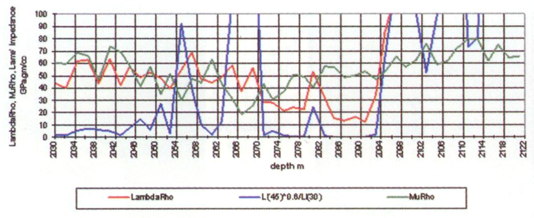
This spectacular result can be seen on the following log tracks for an Alberta BQ gas well in the very low rigidity shale (2063m to 2070m) capping the gas sand zone shown by the LambdaRho and MuRho cross-over between 2070m and 2094m and the low Vs/Vp carbonate below 2094m.

Case Study Log Analysis.

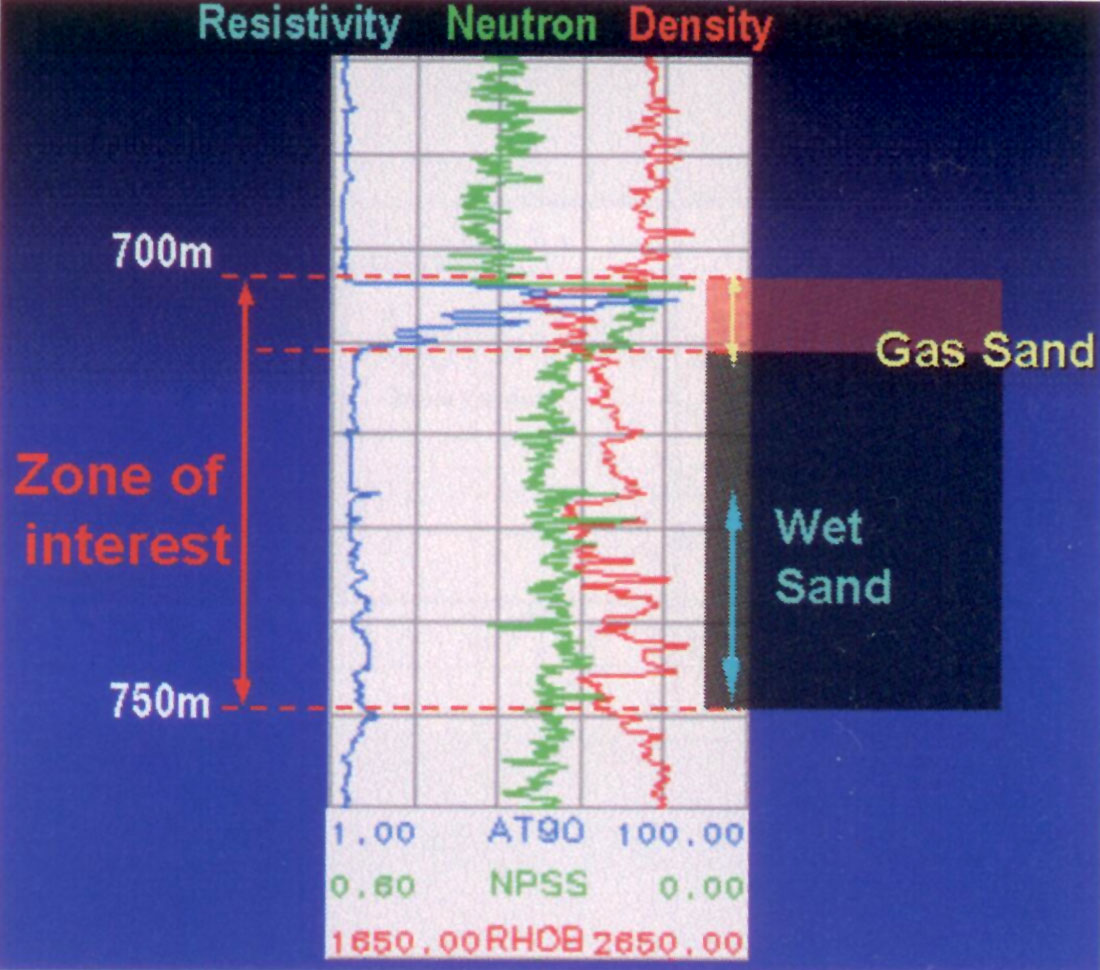
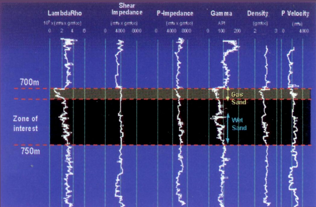
Petrophysical parameters such as lithology, porosity, and fluid saturations were established from a complete log suite for the case study as shown in figure 17. The combined resistivity with neutron density crossover indicates two sands within the zone of interest; a 10m upper gas sand just below 700m and a lower wet sand (below 725m) with marginal gas saturation (fizz gas) as shown by the neutron density approach. Beyond identifying good porosity sand zones from low impedance shale, distinguishing economic gas from “fizz water” is the main challenge for 3D seismic and AVO in the case study area. The improved ability to distinguish gas from wet sand and lithology using Lamé parameters for this Viking sand case study is shown in figures 10a and b, in the previous section on “Log analysis motivation and interpretation templates”. The λ vs. μ and λρ vs. μρ cross-plots show clear clusters that identify the various sand, silt and shale lithologies, as well as showing a clear separation between gas and wet “fizz gas”. Understanding the cross-plot differences between a Lambda-only fluid effect compared to LambdaRho with the advantage of a density influence, shows how the sand zone gas/water saturations may be estimated to better distinguish “fizz water”. The sonic (P and S), density and gamma logs are also shown in depth in figure 18. The lowest λρ values as well as a crossover of λρ < μρ curves (not shown) clearly identify the gas from wet sands, whereas the P and S impedance curves are less discriminating. These low λρ gas zones are the lowest in the whole logged interval, unlike the P impedance and so λρ is an excellent match to the density-neutron crossover data for gas identification as shown in figure 17.

Case Study Seismic walkaway VSP and 3D AVO Inversion for Lamé Parameters.

Awalkaway VSP provides a real seismic data set for calibration of surface AVO, as well as the evidence of a quantifiable AVO response (Downton, Goodway & Chen 1998, 1999). This surface to borehole VSP seismic method has a number of advantages in that a VSP is a controlled experiment where the results are directly tied to well logs in depth and time, so that it is possible to quantify the reliability of the different AVO methods. In addition, the geometry and the angle of incidence are known along with the background Vp/Vs ratio, something that has a high degree of uncertainty when dealing with surface seismic. As the 3D surface seismic was also acquired and processed in a similar fashion to the VSP, so a direct comparison to calibrate and quantify the various AVO inversion results with the VSP data is described below.

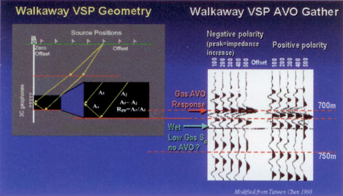
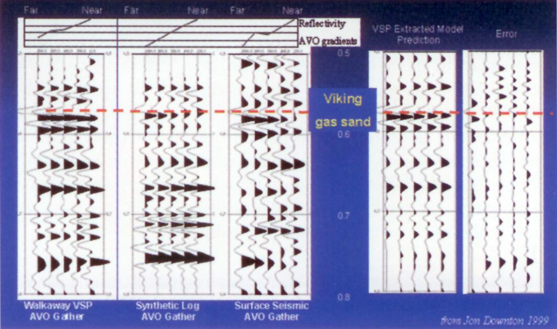
Figure 19 shows the basic walkaway VSP geometry designed for the AVO analysis. Source and receiver locations are schematically shown by flags and triangles respectively, with the source offsets (distance between the source and the surface location of the wellbore) from 100m to 500m at 100m intervals in addition to the full level recorded zero-offset. Through check-shot and sonic log guided ray-tracing, the incident angle at the zone of interest was found to range from 0° to 40° for the largest offset. An amplitude preserving processing flow was designed and applied to both VSP and surface data, resulting in the VSP “AVO gather” response shown in figure 19.

The basic processing sequence followed was to perform an AVO extraction on both the P-wave surface and VSP seismic data as well as the VSP P-S converted wave VSP data to obtain direct estimates of P and S impedance reflectivities. A modified equation to extract P and S reflectivities (Gidlow et al. 1992, Fatti et al. 1994) is used with the last term for small ρ contrasts being ignored, as shown in the previous section on reflectivity equations. This approach was chosen in preference to the various Lamé forms of the Aki and Richards equation (also shown in the reflectivity equations section), as they are not yet in common industry practice for AVO attribute extraction. Having extracted the P, S reflectivity sections, the next step is to obtain Ip and Is through inversion. Finally by using the Lamé moduli to impedance relationships given above, the extraction and transformation to λρ and μρ is obtained.

The VSP P-wave AVO and surface seismic gathers are compared to log based forward modelling in figure 20. An excellent calibration of VSP to surface seismic was achieved as can be seen in the rightmost VSP data to model miss-fit error panel in figure 20.

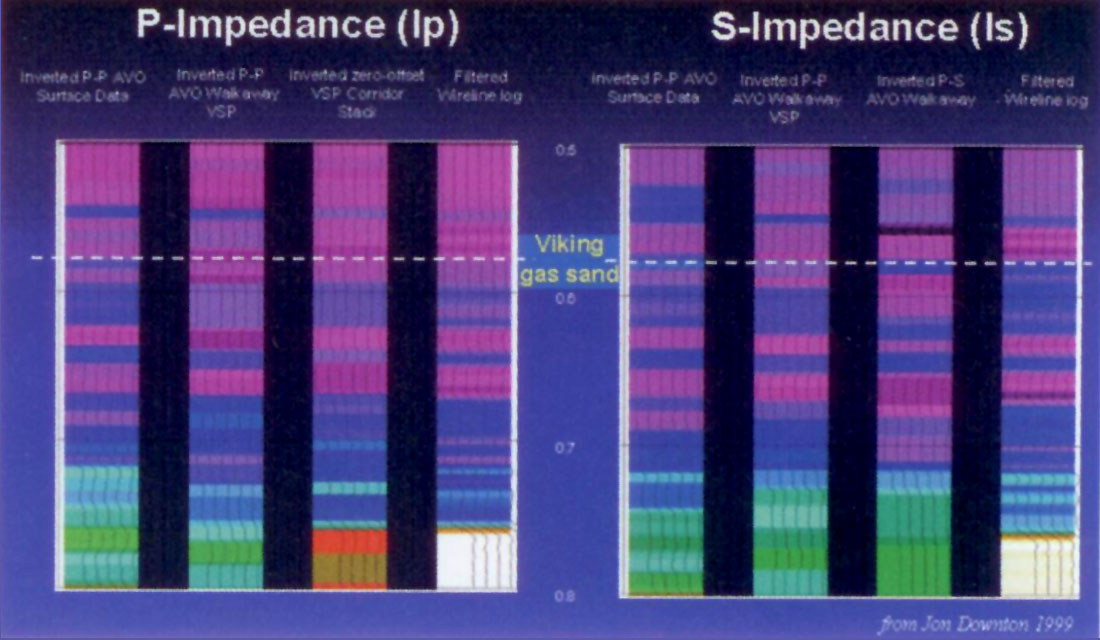
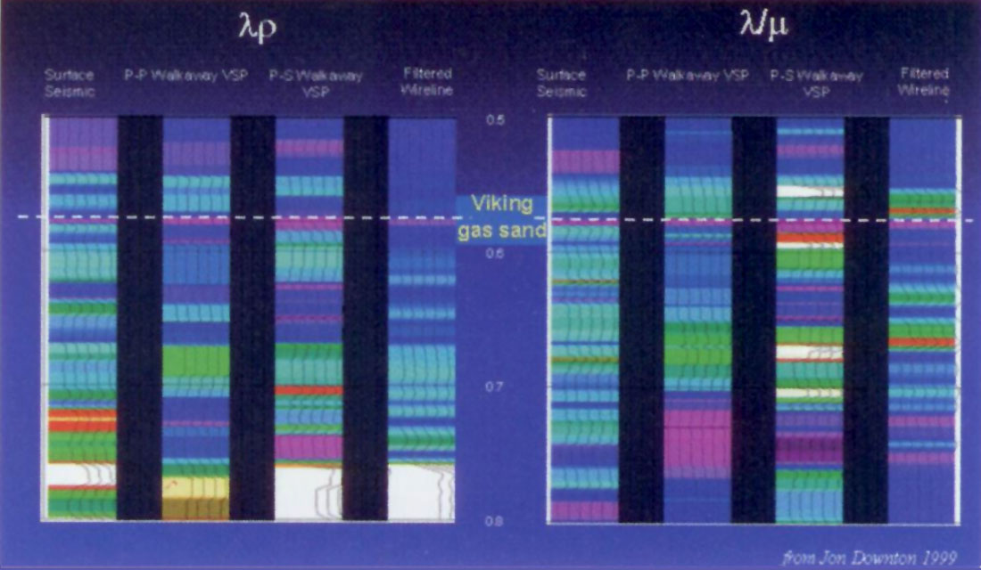
The P and S reflectivity traces extracted from the VSP and surface seismic gathers were inverted using a sparse spike inversion algorithm to get P and S impedances. These values were then crossplotted with the wireline log information showing a reasonable overall correlation (see Downton et al 1999). Qualitative comparisons between P, S impedances and λρ and λ/μ ratios are shown in figures 21 and 22. The leftmost P impedance panel in figure 21 compares surface AVO data to the equivalent VSPAVO and zero-offset VSP inversion with the log impedance. Though the overall match is reasonable the actual gas sand zone is not obvious on any of the panels, being of slightly higher impedance than the background shales. The rightmost S impedance by contrast, shows a strong increase for the gas zone in both surface and VSP P-P, P-S converted wave inversions, that is in agreement with the log data. However a clear increase in shear impedance alone at the Viking level does not distinguish the gas sand from the lower wet sand zones, as shear-waves have a minimal response to fluids. Figure 22 on the other hand shows an unambiguous and very well resolved Viking gas sand zone having the lowest λρ and λ/μ ratios compared to the lower wet sands and encasing shales.

The last set of figures from 23 to 26, compare standard 3D seismic sections and maps of P, S impedance based AVO inversion to the equivalent Lamé parameters and λρ versus μρ cross-plot polygon based methods, as previously described. Stacked amplitudes on the standard 3D seismic line at the Viking zone as marked in figure 23a do not distinguish the gas sand. The equivalent λρ section in figure 23b clearly isolates the Viking gas sand from both encasing shales and the lower wet sand zone in the following trough, shown as the wiggle overlay of the migrated stacked section. The 3D map display in figures 24a and b, of the Viking gas sand horizon with the production results of three wells, show extracted AVO attributes based on P, S impedances (24a) compared to LambdaRho (24b). The impedance-based attribute identifies good gas sand porosity (red-yellow areas) at all three wells and this was the reason these wells were drilled with only one of them (lower left corner) being economic. The LambdaRho attribute map (figure 24b) however, shows a clear grading between the three wells with only the economic well having unambiguously low values. Interestingly both the poor gas well to the top right (watered out within only a month of production) and the D&A well had marginally low gas saturations that are clearly distinguishable from each other, as well as the economic producer.

The final two pairs of figures 25a,b, and 26a,b, show AVO cross-plots for λρ, μρ based polygons compared with a P, S impedance based linear “fluid factor” cut-off, to isolate only the anomalous gas zones from wet sands and shales. The best gas zone λρ, μρ “polygon 1” in figure 25a, is based on the log crossplots shown before in figure 10 and is more discriminating than the linear impedance- based cut-off shown as a white dashed line. The seismic points identified by this “polygon 1” clearly map onto the economic up-dip gas accumulation in figure 25b. Figure 26a shows the same cross-plotting approach for the wet or marginal gas sand “polygon 2 fizz water” prediction, again based on the logs in figure 10. The points identified from this “polygon 2” template map predominantly onto the D&A “fizz water” well and the marginal gas producer in figure 26b, showing the improved gas sand versus wet sand detection of the λρ, μρ approach for surface seismic.

Conclusions

1. Improved petrophysical understanding of rock properties using orthogonal Lamé parameters λ (pure incompressibility) and μ (rigidity) over conventional Vp, Vs or moduli-based analysis.
2. Greater physical insight into rock properties for pore fluid versus lithology discrimination by isolating the Lamé impedances λρ, μρ from the seismic reflectivity response.
3. Easier AVO cross-plot cluster isolation for a more sensitive λρ, μρ lithology stack and for potentially separating fluid saturation effects.
4. A new λ/μ ratio versus λρ-μρ difference cross-plot showing lines of consistent lithology/porosity with fluid saturation (gas vs wet zones) altering the lithology line’s slope.
5. The sensitivity of λρ to fluids has the potential to distinguish economic gas zones from fizz-water as shown by quantitative inversion and calibration of surface and walkaway VSP data.
6. A direct relationship of AVO-derived Lamé parameter λ to the Biot-Gassmann equation.

Acknowledgements

As so much of this paper includes the work and ideas of a number of people (as well as a lot of fruitfully stimulating discussion) I acknowledge the key individuals below who were involved in the development, over the past six years, of the Lamé parameter approach to AVO.

From PanCanadian: Taiwen Chen, Dan Cieslewicz, Dave Cooper, Jocelyn Dufour, Nilanjan Ganguly, Mark Harper, Irene Kelly, Guoping Li, Andrew Lowe, Drew MacGreggor, Dave Mackidd, Holger Mandler, Alli Marshall, Doug Neilson, Ann O’Byrne, Brian Rex, Robert Riddy, Mantu Sihota, Ian Shook, Garth Syhlonyk, Gordon Uswak, Paul Young, Weimin Zhang.

From outside of PanCanadian: Jon Downton and Yongyi Li (Scott-Pickford), Dave Gray (Veritas DGC), George Smith (University of Cape Town), Brian Russell (Hampson & Russell). Finally I wish to thank the Recorder editors, Satinder Chopra and Oliver Kuhn for their initiative to publish as well as their encouragement and amazing patience in getting me to write this article.

These eleven articles represent some of the outstanding technical work being done in our field. We trust this issue will provide you, our readers, stimulating reading, inspire you in your own technical work, and perhaps challenge you to submit an article for a future issue of the RECORDER.

Keep in mind that you still have the September 2001 RECORDER to look forward to, the second part of the “Special Issue”, and it will contain 12 more excellent articles on a variety of topics.