AVO Attribute Analysis on a Class I Clastic Reservoir

This paper examines the usefulness of cross-plotting, as a visualization tool, in helping to understand the relationships between different AVO stacks and the presence of hydrocarbons. In particular, this paper will examine a methodology to identify Class I AVO anomalies using the family of AVO stacks based on Smith & Gidlow's 1987 paper (reference 3); namely the delta-S over Sand delta-P over P stacks. This paper will focus on a Class I anomaly (Rutherford, reference 2) for which, when the reservoir is gas filled, the zero offset reflection amplitude is positive and the reflection amplitude decreases with offset in a stronger fashion than other regional reflectors.

We often get the question "Why do AVO? What is it adding to my interpretation? We are successful enough drilling on bright spots." A Class I anomaly is an excellent candidate for doing an AVO analysis. The gas response of this type can be quite ambiquous on the poststack section. The amplitude should dim but this could also be a result of lithologic changes or tuning, to name just a few other factors. By doing an AVO analysis some of this ambiguity can be removed. Our preference in doing such an analysis is to work with a pair of AVO stacks such as the delta-P over P stack and the delta-S over S stack. The second stack provides extra information which can help make the interpretation more unique. In mature exploration areas the question as to be asked, "What are we bringing new to the analysis that others have not done before?" It is the contention of this paper that AVO is one such tool.

The particular example that this paper will look at is a Bluesky sandstone reservoir from the Alberta/British Columbia border in Canada. The Bluesky is of Cretaceous age and overlays the Gething and Cadomin which rest unconformably on the Triassic. The Bluesky to Triassic isopach can change significantly, introducing tuning issues. The original exploration play was to drill on Triassic highs. In this area the Bluesky is at a depth of about a, 1000 meters and is higher impedance than the overlying shale, implying a Class I AVO anomaly.

This paper is going to focus on a regional line (figure 1) chosen because of its good data quality and varied well control. The line was acquired with a dynamite source, a 10m group interval and a 80 m shot interval with a maximum offset of 1550 meters. The Bluesky shows up as the marker at 750 milliseconds. This line had a good signal to noise ration up to 80 Hertz at the zone of interest. Good quality data is needed in this area to accurately resolve thin gas sands in the order of 3 to 6 meters gross thickness. We have tried a similar analysis on older data from late 70' s with a larger group interval, but with disappointing results.

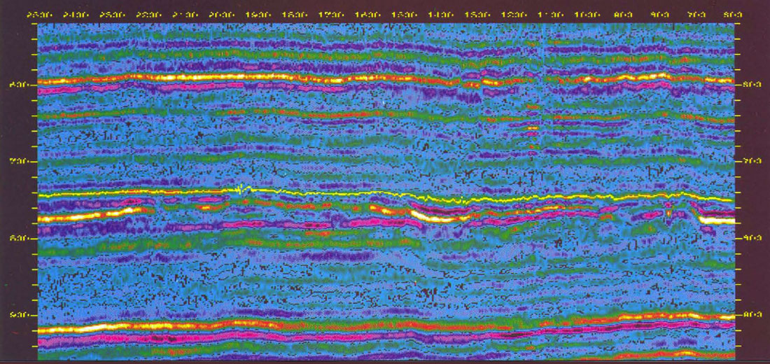
Four wells intersect at this line. Well A, at shotpoint 2400, encountered a regional wet Bluesky sandstone. Well B at shotpoint 1800, encountered a thick 12 m gas filled Bluesky sand reservoir. Likewise, Well C at shotpoint 1400, encountered a gas sand, but with only a meter of thickness. Lastly, well D at shotpoint 700, encountered a wet Bluesky sand. Originally, the wells where drilled based on structure. This was the rationale for both Well B and D, one of which was wet.

The objective of the project was to determine if AVO could be used to determine the fluid content of the reservoir prior to drilling.

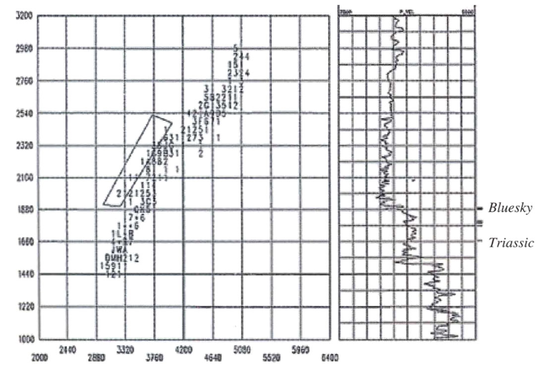
Figure 2 shows a gas well in the area. On the right hand side of the figure is the sonic log. The Bluesky top is marked. For this particular well, there was both p-wave and s-wave velocity information. This is cross-plotted on the left hand side of the figure with the p-wave velocity on the horizontal axis and s-wave velocity on the vertical axis. There is a clear regional trend (mudrock line), as well as some anomalous values which depart from this trend. These anomalous values were highlighted by drawing a polygon around them. The highlighted points can then be referenced back to the sonic log, on the right by displaying tick marks on the depth axis next to the sonic log. From this it can be seen that the anomalous values in cross-plot space correspond to the gas filled Bluesky reservoir on the sonic log. This suggests that the fluid stack methodology advanced by Smith & Gidlow (reference 3) should be able to act as a gas indicator for this particular play.

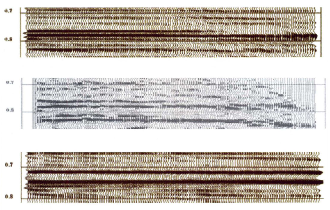
To understand what the seismic response of this should be, forward modeling was performed on both a gas well and wet well in the area. The modelling was performed using an elastic modelling scheme with the acquisition geometry of the template line. The top panel in figure 3 is the modelled AVO response for the gas reservoir using the p-wave, s-wave and density information from Well B. The Bluesky event, the peak at 780 milliseconds, goes from a strong amplitude at zero offset to zero amplitude at 1000 meters. The middle panel in figure 2 shows the actual seismic data from the line at that location. The seismic data is mixed in both the cdp and offset dimensions to improve signal to noise for display purposes. The Bluesky event, which is the peak at 770 milliseconds, decreases with offset just like the synthetic model The bottom panel in figure 3 is that of a synthetic cdp model based on a wet Bluesky reservoir. The Bluesky, which is the peak at 710 milliseconds, remains constant with offset. The reader might note that the character at the Bluesky from the wet model is considerably different than that of the gas model. This is because the isopach between the Bluesky and the Triassic changes quite considerably and the two reflectors tune. This is an additional complication in the AVO analysis.

Next, both delta-P over P and delta-S over S AYO stacks were generated for this line. The top panel in figure 4 is the Delta-P over P stack. The Bluesky amplitude (around 750 milliseconds) varies across the line in a manner consistent with the well control At well A, the amplitude is quite high. In the area between well Band C the amplitude decreases in a manner consistent with a gas reservoir. halfway between well C and well D the amplitude of the Bluesky is again quite high. The fact that these amplitude variations match the well control seems quite encouraging, but other factors could cause this behavior such as tuning or lithologic changes.

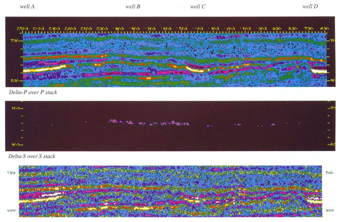
The delta-S over S stack can help answer this question (middle panel of figure 4). The delta-S over S stack should not react to changes in fluid content but should behave in a similar fashion to the delta-P over P stack in the case of lithologic changes and tuning. In this case the amplitude of the Bluesky on delta-S over S stack remains quite consistent throughout the line. This suggests that the lateral changes we see on the delta-P over P stack at the Bluesky level are a result of fluid content.

To help quantify this change. the amplitude of the peak from the Bluesky horizon was extracted from the delta-P over P stack and the delta-S over S stack and cross-plotted. The delta-P over P-reflectives are plotted along the vertical axis and the delta-S over S reflectives along the horizontal axis. The origin is in the middle. Cross-plots were created at two points along the line; one over the gas well at location B and one over the wet well at location A. The cross-plots for each of these two situations tightly cluster and are shown superimposed in figure 5.

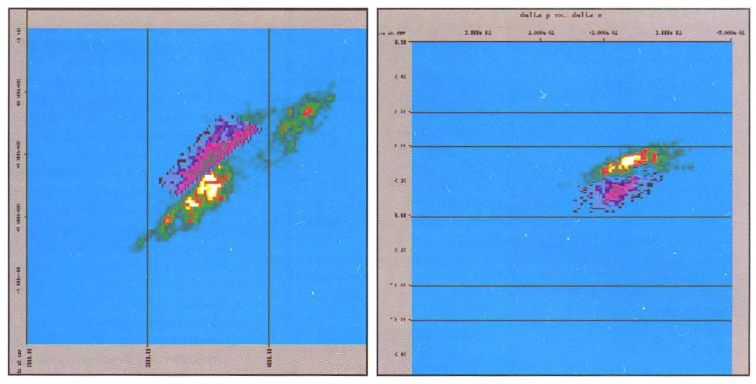
The cluster associated with the gas well (grey cluster) is closer to the zero axis compared to the cluster from the wet well (white cluster). There is little movement between the two clusters along the horizontal axis. This is consistent with the theoretical gas response. The presence of gas should lower the p-wave velocity dimming the delta-P over P peak reflection. The S-wave velocity should largely be unaffected implying that there should be little change in the delta-S over S stack. This is indeed the case.

Since the two clusters occupy different area' in the cross-plot space it should be possible to design a filter to emphasize the data points in the gas area for the whole line. This was done by picking a mute polygon similar to the procedure followed earlier for the well log cross-pial. The results of this are shown in the lower most panel in figure 4. There is an excellent correlation with the well control. The two wet wells show no response, the thick gas well (well B) shows a good response and the thin gas well is just on the edge of the anomaly.

This analysis is sensitive to what information we cross-plot. In this case, we crossplotted the peak amplitude extracted along the Bluesky horizon from the two AVO stacks. Often in thin, tuned reservoirs, phase and character information are as significant as the amplitude information. For example, we have found the AVO anomaly can show up half a leg up or down from the reservoir as a result of tuning. In order to get good results, it is essential to understand what attributes should be extracted to best describe the anomalous behavior. Forward modelling can help one understand these issues.

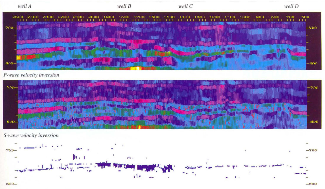
One way we have tried to address this is by doing the analysis on post-stack inverted AVO stacks. By doing the analysis on inverted data the results are less sensitive to wavelet character and tuning. In this case we inverted the delta-P over P stack into a P-wave velocity inversion (figure 6, top panel) and the delta-S over S stack into as-wave velocity inversion (figure 6, middle panel). A sparse spike inversion algorithm was employed using the well information to constrain the solution.

The P-wave velocity inversion shows a relative drop in velocity at the Bluesky level (750 milliseconds) around the gas wells. However, the S-wave velocity inversion shows the Bluesky velocity to remain quite consistent all across the line. Once again, a cross-plot analysis was performed to quantify the extent of the anomaly (figure 5b). The P-wave velocity is shown on the horizontal axis and S-wave velocity on the vertical axis. The origin is in the lower right hand corner. The analysis is performed over a 100 millisecond window centered on the Bluesky over the entire line. Most of the data points fall along a straight line which we defined as the mudrock line (reference 1). There are some anomalous points above the line similar to the well log cross-plot in figure 2. These points have a lower P-wave velocity, consistent with a gas reservoir. A polygon was used to select these points. These points were then displayed in the lower panel on figure 6 giving an excellent correlation with well control.

There are a number of strengths with this last approach: no horizons need to be picked nor amplitudes extracted, tuning and wavelet character are less of an issue. The biggest drawback with this approach is that one must have a good quality delta-S over S stack. Often this stack has a poorer signal to noise ration than the delta-S over P stack. This becomes significant when we invert the two results. If the delta-S over S stack is significantly nosier it will react to the constraints differently than the delta-P over P, stack giving a slightly different low frequency trend. The difference in the trends will then dominate the cross-plot solution.

In conclusion, AVO stacks can provide extra information helping to make the interpretation more unique. It is information free for the interpreter to exploit. The challenge with each play, just like with a conventional interpretation, is to discover which attributes best describe the geology while using the well control as a constraint. Once this is determined one has a powerful predictive tool.