AVO Crossplotting Revisited: A Practitioner’s Perspective

The development of AVO crossplot analysis has been the subject of much discussion over the past decade and has provided interpreters with new tools for meeting exploration objectives. Papers by Ross (2000) and Simm et al. (2000) provide blueprints for performing AVO crossplot interpretation. These articles refer to the Castagna and Swan (1997) paper which laid the foundation for AVO crossplotting. The AVO classification scheme presented by Castagna and Swan, which was expanded from the work of Rutherford and Williams (1989), has become the industry standard. Castagna and Swan also investigated the behavior of constant Vp/Vs trends, concluding that for significant variations in Vp/Vs many different trends may be superimposed within AVO crossplot space, making it difficult to differentiate a single background trend. A misapplication of this concept has been to infer a direct correlation between these changing background Vp/Vs trends with rotating intercept/gradient crossplot slopes (what Gidlow and Smith (2003) call the fluid factor angle, and Foster et al. (1997) the fluid line) observed in seismic data. The central question of this paper is: when is this background trend (or fluid line) rotation a representation of real geology and when is it a processing-related phenomenon? To answer this question I review the theoretical expectations regarding rotating AVO crossplot trends, the role of seismic gather calibration (or lack thereof), and the value of various compensating methods. Furthermore, I investigate the appropriateness of using constant Vp/Vs lines in a crossplot template by examining both the mathematical and modeled AVO crossplot responses which incorporate an established compaction trend. I conclude that when exploring in a reasonably compacted environment (Vp/Vs ratios of 1.6-2.4) a relatively small range of fluid angles (background trend rotations) can be expected. Large variations of fluid angle observed in seismic data can be attributed to the difficulty in preconditioning gathers for AVO analysis.

AVO Crossplot Rotations

The key value of AVO crossplot interpretation is the ability to differentiate population outliers relative to background trend points within crossplot space. Incorporating direct hydrocarbon indicators (DHIs) via crossplotting can play a significant role in minimizing the risk associated with an exploration play. The stability of the background trend (fluid angle) can have an impact on what is being interpreted as anomalous, be it fluid or lithology induced outliers. Castagna and Swan’s (1997) Interpreter’s Corner article concluded that many background trends can be erroneously superimposed in AVO crossplot space, particularly if too large a depth range is brought into the interpretation window. This presents difficulties when performing crossplotting analysis, particularly as it pertains to non-uniqueness. For a given anomaly (population outliers) an interpretation of an increase in Vp/Vs (due to a superimposed background trend) can be just as feasible as a decrease in Vp/Vs (due to a fluid response or coal) dependent upon the choice of background trend. The Castagna and Swan crossplot template, seen in figure 1a, is often used in the literature to explain crossplot behavior observed in seismic data. However, the constant Vp/Vs lines used in the design of this crossplot template do not reflect most worldwide compaction trends and established empirical mudrock line relationships. Figure 1b highlights how constant Vp/Vs lines cut across a given mudrock line only within a limited range. Outside these overlap zones the constant Vp/Vs lines would be considered physically unrealistic. A follow-up Interpreter’s Corner article by Sams (1998) also questions the appropriateness of using these constant Vp/Vs trends in crossplot templates. Sams demonstrates that constant Vp/Vs lines approach a mudrock line relationship only at very high P-wave velocities.

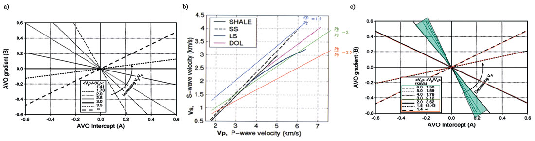
Castagna et al. (1998) address this very concern in their expanded follow-up article. Figure 1c shows the rotation of the intercept/gradient slope when a linear Vp versus Vs trend is taken into account in the creation of the crossplot template. The result is a less dramatic rotation of background trend rocks within moderate ranges of Vp/Vs ratios. The AVO crossplot rotation effect can be problematic for interpretation only when low velocity unconsolidated materials (and their associated high Vp/Vs ratios) are encountered. An example from the Western Canadian Sedimentary Basin (WCSB) illustrates the significance of this result. Most reservoirs in the WCSB have velocities on the low end of 2500m/s (clastics) and at the high end of 6000m/s (carbonates). Within this velocity range Vp/Vs ratios of 1.6-2.5 encompass most background trend rocks and this places their AVO responses within the green background trend highlighted in figure 1c. Another factor to consider during the interpretation of crossplots is the signal-to-noise ratio (S/N) issues which tend to broaden the intercept and gradient (I/G) reflectivity points within crossplot space into oval distributions (Simm et al., 2000). This seismic noise acts to further blend the background trend lines together into a singular cloudy trend. Therefore, since depth dependent fluid angle variations are typically small and often embedded within seismic noise, larger temporal windows can be brought into AVO crossplot space when searching for AVO anomalies in the WCSB.

The term rotation is used frequently in this article to describe observations made in AVO crossplot space. A more appropriate term to use is apparent rotation, as points in crossplot space are not actually going through a true rotation (denoted by I’=I cosθ + G sinθ, G’=- I sinθ + G cosθ ) but instead are being subjected to scaling and/or skewing operations (denoted by I’=k1 x I, G’=k2 x G and I’=k1 x I, G’=k2 x G + k3 x I, respectively).

AVO Modeling

Modeling was performed using a Castagna mudrock line relationship (Castagna et al., 1985) to verify the assertion that AVO crossplot slopes should be comparable when the Vp/Vs trend is depth dependent (i.e. following a compaction trend). In this model (figure 2a) the shallow section contains sands with lower impedance than surrounding shales, the intermediate section contains sands and shales of similar impedance, while the deeper section contains sands with higher impedance. An offset synthetic was created using a zero-phase seismic wavelet of reasonable bandwidth (Figure 2b), and AVO extraction was performed using the Shuey equation (1985).

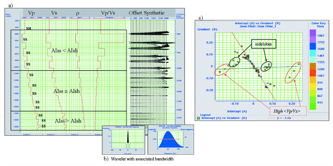
Several things stand out in the AVO crossplot model (Figure 2c). First, there is a relatively tight background trend (red line). Next, there are data points (circled in black) representing wavelet side lobes, not geology. Finally, there is an offset population (circled in red) with a near horizontal slope (i.e. with zero gradient). This model was constructed using background trend rock s (wet/brine) and no hydrocarbon induced responses are included. As with the Castagna et al. (1998) template (Figure 1c) the lower velocities present in this model (i.e. the shallowest sands) represent the transition in the Castagna mudrock line from a matrix supported formation to a fluid supported one. These observations highlight the importance of recognizing where and when potential sources of confusion can be introduced into a crossplotting template.

Since seismic data is a reflectivity attribute (measuring the contrast between impedance quantities) it is helpful to re-express the model parameters as a function of average Vp/Vs change, <Vp/Vs>. In Figure 3, each of the reflectivity interfaces used in Figure 2. AVO Model Example. (a) An AVO model was built using: Vp honouring a compaction trend; Density estimated using the Gardner et al. (1974) equation; Vs estimated using the Castagna et al. (1985) equation. These logs and a seismic wavelet (b) were used to create an offset synthetic. (c) AVO crossplot of the modeled data highlighting: the background trend line; data points associated with wavelet side lobe effects; and rotated data points stemming from the lower velocity reflections. This model is a confirmation the model is identified using the letters A (shallow) through U (deep), along with their corresponding <Vp/Vs>. The same letters identify these interfaces in crossplot space, with the previously noted side lobe effects removed to better visualize the impedance contrasts only. Figure 3a (left, upper crossplot) used the Castagna mudrock line relationship, as seen in figure 2, while figure 3b (right, lower crossplot) repeated the modeling using the Han mudrock line relationship (Han et al., 1986).

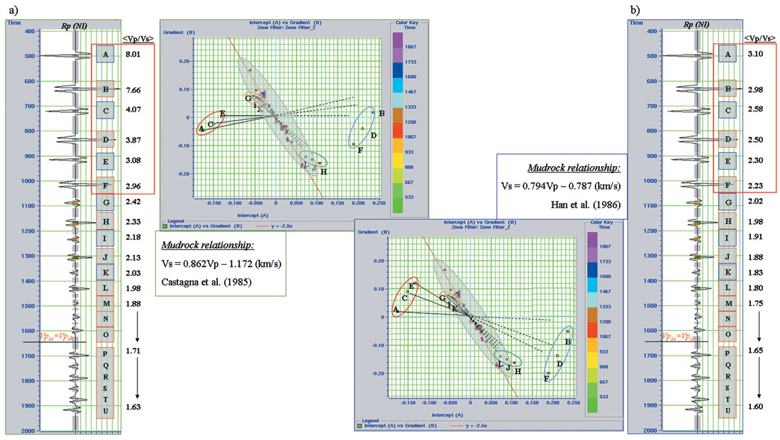
This modeling reinforces the work presented by Castagna et al. (1998) where AVO trend lines are relatively tight in compacted rocks (lower Vp/Vs) and rotate more strongly for unconsolidated sediments (high Vp/Vs) only. The grey polygons in both crossplot spaces are a qualitative approximation of the data point scatter that would take place when seismic noise is introduced. The amount, and type, of noise present in the gathers will have an impact on the size and configuration of this data scatter. The model converges on a well behaved background trend for <Vp/Vs> values below 2.42 using the Castagna mudrock line and values below 2.02 when using the Han relationship. For the lower velocity wet sands in the shallow section, highlighted by red boxes in figures 3a and 3b, the rotation towards anomalous AVO space (Class III/IV response) happens at different rates depending on the magnitude of <Vp/Vs>. Great care should be taken in undercompacted basins to determine the AVO crossplot sensitivities so that population outliers associated with background trend rocks are not interpreted as DHIs. How large a fluid angle variation to expect should be modeled up-front so that comparisons of anomalous population rotations (due to all factors including hydrocarbon, lithology, and/or overpressure effects) are incorporated into the pre-AVO risking. As expected, since the Han relationship was designed using lower velocity sands and shales it yielded the lower and more realizable <Vp/Vs> contrasts for the shallower rocks, and experienced the smaller fluid angle rotation of the two.

AVO Equation

It is possible to investigate how much each component (Intercept and Gradient) contributes to the population rotations observed in AVO crossplot space by looking more closely at the equations governing AVO behavior. Thomsen’s (2002) approximations were used (see equation 1) along with a simple compaction model (i.e. velocity increasing with depth). The following assumptions were made to calculate the acoustic impedance (AI) contrasts: the Castagna et al. (1985) mudrock line was used to estimate the S-wave velocity; Gardner et al. (1974) was used to calculate the density; in the spreadsheet smaller reflection coefficients were identified by simply comparing impedances with similar values (smaller Δdepth) while larger reflection coefficients required contrasting impedances with larger differences (larger Δdepth); as the reflection coefficients (R₀ and R₂ ) were calculated the ΔVp was kept constant, as opposed to holding the fractional change in Vp constant. Note: The curvature term (R₄) was ignored because most datasets do not have the necessary quality long offset (angle) data required to benefit the AVO results, although this trend is starting to change.

Several key insights came from this exercise. First, figure 4a shows that the normal incidence (zero offset) reflectivity amplitudes increase as the P-wave velocity decreases. This illustrates that the intercept term also contributes to the rotation observed in AVO crossplot space. The magnitude of this rotation becomes more significant as the velocity contrast becomes larger. Next, for gradient responses (shown in figure 4b) corresponding to velocities lower than < 2300* m/s a polarity flip takes place. Simply stated, in lower velocity environments peaks and troughs actually can become brighter with offset, an observation noted by Castagna et al. (1997). This goes against conventional AVO quality control (QC) practices/assumptions that all amplitudes should decay with offset, unless hydrocarbon affected. It is important to point out that at these high Vp/Vs values (low velocities) the rocks are closer to being an acoustic medium (shear modulus µ=0) rather than an elastic medium. In areas such as offshore West Africa, and shallow heavy oil plays in the WCSB, contrasting density reflections can provide more illumination into a reservoir than the Vp/Vs contrasts. Three-term AVO (Downton and Chaveste, 2004), or two-term converted wave (PS) AVO (Jin et al. 2000) become more valuable in these instances as they solve for density reflectivity. For this particular example the Vp/Vs vs. Vp crossplot (figure 4d) shows that the crossover in AVO Gradient takes place at approximately Vp/Vs=2.8*. (*Note: This crossover point is very much dependant on the local mudrock relationship as well as the magnitude of the AI contrast. For example, in figure 4b the crossover point for the Q IV (large RC) case is at a higher Vp and lower associated Vp/Vs than the crossover point for the Q IV (small RC)).

The evaluation above supports using large temporal windows in AVO crossplotting analysis to find larger prospective lithologic and fluid outliers as long as it is within a consolidated depositional setting (i.e. Vp/Vs values ranging from 1.6-2.5). This does not follow conventional practice (Castagna et al., 1998) and can be problematic for two reasons: 1) the weaker/subtle population outliers (ex. lower API oil, or hydrocarbons in hard carbonates) may be too subtle to extract from the background trend, and 2) in practice when examining large temporal windows most seismic data does not behave according to this theoretically tight background trend. In the case of the latter I believe the disconnect between theory and practice can be attributed to the difficulties inherent in the data conditioning prior to the AVO extraction process.

Processing for AVO / Calibration

Cambois (2000) defines a processing workflow meant to be AVO friendly simply as “any sequence that makes the data compatible with Shuey’s equation” (or various other Zoeppritz approximation methodologies). True Amplitude, Preserved Amplitude, and Controlled Amplitude Controlled Phase (CACP) are a few examples. Many of these workflows include deterministic and/or statistical corrections calculated by incorporating well logs and/or geologic models. These workflows may comprise larger amplitude corrections, such as geometrical spreading and absorption (Q), or more subtle ones, like angle of emergence and array corrections. Typically these workflows apply time and offset variant corrections in an attempt to compensate for the earth filter. Several authors have discussed at length the difficulties inherent in this process, including Cambois (2001) and Bachrach; Kozlov and Ivanova; Landro and Stavos (2006).

Processing workflows like the one described by Ramos (1998) highlight the need to compare and contrast the AVO behavior after every processing step. Qualitative and quantitative evaluation involving the amplitudes of our primaries is performed to determine if any gradient responses have been altered. Gather difference plots are an interpreter’s best friend when maintaining quality control. Some QC methods need to be more sophisticated in order to quantify any possible changes. For example, the difference of a gather pre- and post-spectral whitening cannot be used because the frequency content of the primaries has been altered too dramatically. In these cases it is necessary to crossplot the AVO attributes, before and after the process to test the response on known population outliers.

The goal of these true amplitude flows is to restore the amplitude (and phase) response to a point where geologic meaning can be inferred. It is important to understand that the gradient behavior (as a function of time) is dependent upon the processing applied to that data. Revisiting figure 4c, we observe that all background trend rocks have amplitudes that decay as a function of offset. In other words, positive intercepts have negative gradients, while negative intercepts have positive gradients (For the sake of simplicity I am generalizing to include only the consolidated rocks, not the rarer low velocity regimes discussed previously). The rate at which these gradients decay can be very much affected by the processing applied, especially when offset varying applications are present. The first check when quality controlling CDP gathers is to verify that the majority (i.e. nonanomalous) of the reflection events do indeed decay. This decay should be noticeable over the angle of incidence range of 0-40 degrees, and then the amplitudes can sharply increase again as they approach the critical angle. Note: this means that for shallow data the amplitude decay will happen relatively quickly over a given offset range compared to the decay that will be more gradual deeper in the section over the same offset range. Another way of expressing this is: as time increases the angle of incidence range decreases.

A common misunderstanding is to assign a correlation between the rotating intercept/gradient crossplot slope observed in seismic data and the rotating background trends as described by Castagna and Swan (1997), shown in figure 1a. Given the potential for inaccurate time-variant gradients within seismic data, this is troublesome for the following reasons: a) figure 1a is not a realistic representation of how crossplot populations should behave, whereas figure 1c is; and b) despite our attempts, most processing flows do not fully account for all of the complex earth filtering of the data. Apparent rotations in crossplot space (static or time variant), measured on real data, may actually be telling us more about how much residual earth compensating corrections are still required rather than representing actual geologically meaningful Vp/Vs trend variations. The issue is further complicated when the effects of noise are considered, as discussed by Cambois (1998).

Alternative Calibration/Interpretation Techniques

What can be done if time and resources are insufficient to apply a calibrated AVO workflow prior to an AVO analysis? There are many common practices that provide viable workarounds to the calibration uncertainty issue. One of the most well known approaches is the Geogain methodology, introduced by Gidlow et al. (1992). In this approach a Fluid Factor stack is calculated by subtracting the intercept attribute (the P-wave reflectivity – denoted R_p or ΔI/I ) by a scaled version of the gradient attribute (the S-wave reflectivity – denoted R_s or ΔK/K ) (equation 2).

The smoothed time-variant and spatially-variant scalar, g(t), is applied to the gradient attribute post AVO extraction. This scalar initiates a rotation in crossplot space whereby one-to-one correlated R_p and R_s points cancel out and all uncorrelated points (i.e. anomalous fluids and/or lithologies) are highlighted in the fluid factor attribute. Buried in the g(t) scalar are both the mudrock line contribution (Smith and Gidlow, 1987) as well as the seismic calibration term. This calibration term is often misinterpreted as a geologically induced crossplot rotation. Since all the low frequency time-variant background trends have been collapsed onto a one-to-one line (45 degrees) crossplotting the intercept attribute along with the scaled gradient attribute provides the interpreter with the ability to crossplot larger time windows. Note: This assumes that the processing induced time-variant gradients (i.e. time variant rotations in crossplot space, or “ residual calibration”) are comparable to the low frequency g(t) scalar trend. For example, if the ΔF scalar design window is too large not all of the time-variant fluid angle rotations may be removed, but too small a window could rotate anomalous data populations (i.e. potential reservoirs) into the background trend. Despite being able to bring in larger windows this does not mean that vertical (temporal) windowing is necessarily preferred to horizontal (spatial) windowing. Evaluating a formation across a large horizontal crossplot window is the preferred way of inferring lateral facies/fluid variability as rock properties may be changing too rapidly with depth for fair comparisons to be made. Each reservoir has its own unique noise, structural, and/or lithologic elements and several crossplot trial and error iterations may be required to best illuminate anomalous population outliers. The

Geogain methodology, and others fashioned after it, can produce results comparable to having performed a calibration to a set of gathers (when parameterized correctly).

One of the best ways to ensure the optimum calibration of seismic data is to perform an inversion (Cambois, 2001). During the inversion process the seismic reflectivity data is scaled to match the well log reflectivity, therefore anomalous time-variant gradients are also scaled appropriately. Furthermore, interpreting inversion crossplots may be easier as a result of adding the time-variant low frequency log trends to the data. Overlapping data trends present in AVO reflectivity space are now separated into discrete geologic intervals. This is the benefit of moving from a differential property (changes of one quantity relative to another) into a layer property.

Finally, there is much literature devoted to developing more sophisticated attribute displays derived from AVO crossplot space. The fluid factor represents the perpendicular distance of anomalous data points relative to the background trend. More complex segregation techniques (ex. color scheme manipulations, 3D crossplotting) have produced stack and/or map representations of fluids, porosity, and lithology – just to name a few. While these approaches have merit, the key thing to remember is that these attributes can be automated and may not always represent the true nature of what is happening with the data. Any crossplot derived, or crossplot related, attribute should always have an associated crossplot displayed alongside of it. This requirement is as fundamental as evaluating the gathers that have produced any stack/AVO/inversion related anomaly. When dealing with these attribute choices remember that sometimes less is more. Why not simply interpret the crossplot space itself, while simultaneously highlighting the fluid, porosity, and lithology populations/trends in one pass, rather than dealing with a myriad of attribute sections which require cross referencing in order to tell the whole story?

Application

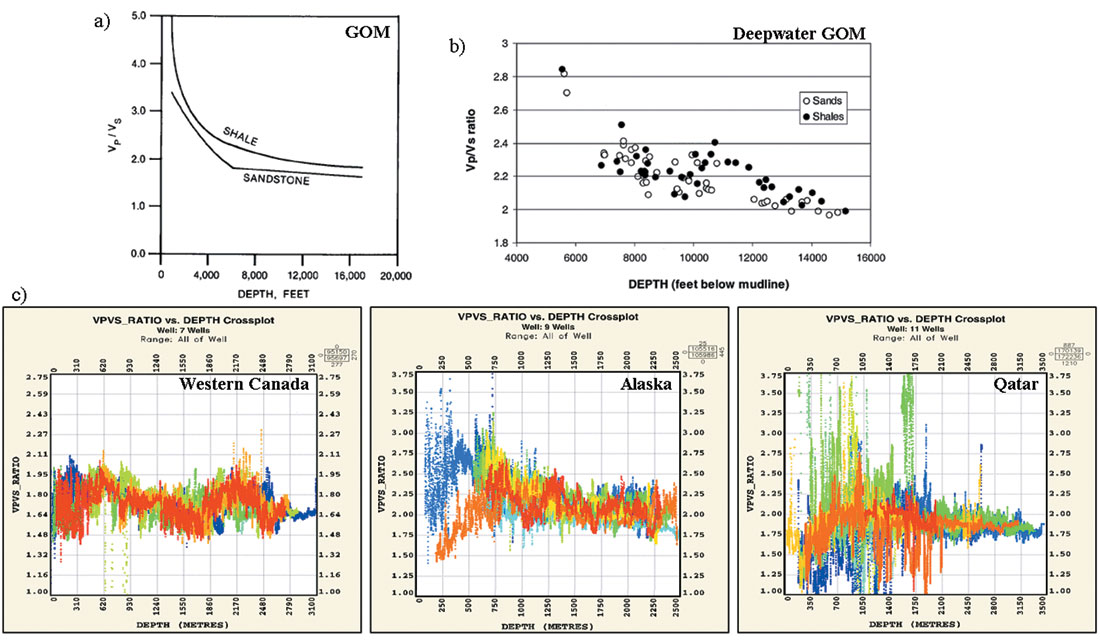
An important aspect of any AVO study is to understand the AVO sensitivities and/or limitations within the local environment. It has been demonstrated in the discussion above that one would expect to see noticeable rotations of the background trend within AVO crossplot space in lower velocity regimes only. An evaluation of several diverse basins around the world was performed to see how each regional AVO crossplot space behaves, and to find where crossplot rotations could be present within the AVO background trend. Figure 5 shows that for the vast majority of target depths within the studied areas the Vp/Vs ratios were sufficiently low (2.25 or lower) such that the degree of rotation present in the AVO fluid angle is subtle. Potential confusion or non-uniqueness errors that could arise during the AVO analysis process are restricted to the near surface only in these areas. In the GOM examples, at depths of ~6000 ft. or shallower, the rapid sedimentation rates associated with younger basins present a risk for complicated AVO crossplot rotations, as shown in figure 5 (a) and (b). It is important to note that well logs in the shallower more unconsolidated zones can suffer from bad hole data and extra care must be taken before incorporating them into an AVO study. This is apparent in both the Alaska and Qatar Vp/Vs crossplots, in figure 5c.

Conclusion

AVO crossplotting techniques and applications have evolved over the last decade. Deciding which AVO crossplot template to apply in a given play requires a petrophysical understanding of the environment. For instance, when logs are indicating a well compacted environment (Vp/Vs ratios of 1.6-2.4) a relatively small range of fluid angles (background trend rotations) can be expected in the seismic data during the course of an AVO investigation. This can allow for more latitude in crossplot analysis strategies. For example, larger time windows can be brought into crossplot space than previously considered. It is important to understand how calibrated the seismic data is beforehand when performing crossplot analysis. Background trend rotations observed in the seismic, as a function of time/depth, are typically not representative of the local geology. The AVO fluid angle experiences dramatic variations only in extremely low velocity environments , often producing polarity shifts in the AVO gradient. The calibration process can be difficult; however, simple and effective alternatives are available. For most datasets, sticking to an AVO friendly processing flow and applying a time-variant fluid factor correction after AVO extraction is a practical workaround to a rigorous calibration process. Finally, although it may be tempting to skip the AVO crossplot analysis altogether to perform an inversion (the ultimate form of calibration) it is important to be cautious and not trust the inversion implicitly. Any anomalies identified by an inversion analysis should always be confirmed in AVO crossplot space as well as reviewed on the input gathers themselves to rule out other, less geologically driven, causes.

Acknowledgements

Special thanks to David D’Amico, Hugh Geiger, and Brian Russell for helping this article to evolve through the various stages of development.