AVO Processing: Myths and Reality

Summary

AVO processing is meant to make the input data compatible with Shuey’s equation. This task is extremely difficult due to the overly simplistic formulation of the problem compared with the complexity of the real physical experiment. Fortunately, the advent of elastic impedance has made it possible to relax some of the processing requirements. Some major concerns (such as amplitude balancing and NMO-stretching) have become almost irrelevant, while others that were often overlooked (such as residual-NMO and multiples) have become critical.

Introduction

Although preserved amplitude processing is a clear requirement for AVO studies, such a processing sequence is not uniquely defined. In particular, “preserved amplitude” has a different meaning for land and marine data. One possible definition could be: Any sequence that makes the data compatible with Shuey’s equation (if this is the model used for the AVO analysis). The simplicity of this definition should not hide the Herculean nature of this task!

Shuey’s equation can be used in two alternative ways: Either directly on the pre-stack samples (the standard AVO approach), or after stratigraphic inversion of angle-limited data (the elastic impedance approach of Connolly, 1999). These two methods share many similarities: They use the same approximations of the wave equation (e.g. Shuey), the same geometry (incidence angles) and the same input data (NMO-corrected, pre-stack time migrated). They differ, however, in the model: The elastic impedance approach is more permissive because it allows for wavelet variations with offset (Cambois, 2000a).

Influence of generic noise

Without going into the specifics of various types of noise, the least-squares formalism provides an analytic expression for any attribute response to generic noise. The stack, for example, is well known to reduce noise in proportion to the square root of the fold. Expressions for intercept (A) and gradient (B) are a bit more complicated (Cambois, 1998), but assuming the range of incidence angles is small enough, their standard deviations can be approximated as:

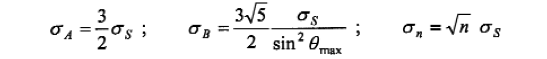
an n^th substack of the full-fold data. From these formulas it can readily be obtained that the intercept is less robust than a half-fold substack, but more robust than a third-fold substack. The gradient standard deviation is inversely proportional to the sine squared of the maximum angle of incidence. Since this number is generally very small, the gradient is clearly unreliable. Figure 1 shows how these standard deviations vary with the maximum angle of incidence (the small angle approximation no longer applies). They are normalized by the stack standard deviation, which effectively removes the effect of fold. The intercept standard deviation is almost insensitive to the maximum incidence angle, while the gradient uncertainty improves with increasing aperture. Note that shear-reflectivity [equal to (A-B)/2] and Poisson-reflectivity [equal to A+B] have the same uncertainty as the gradient.

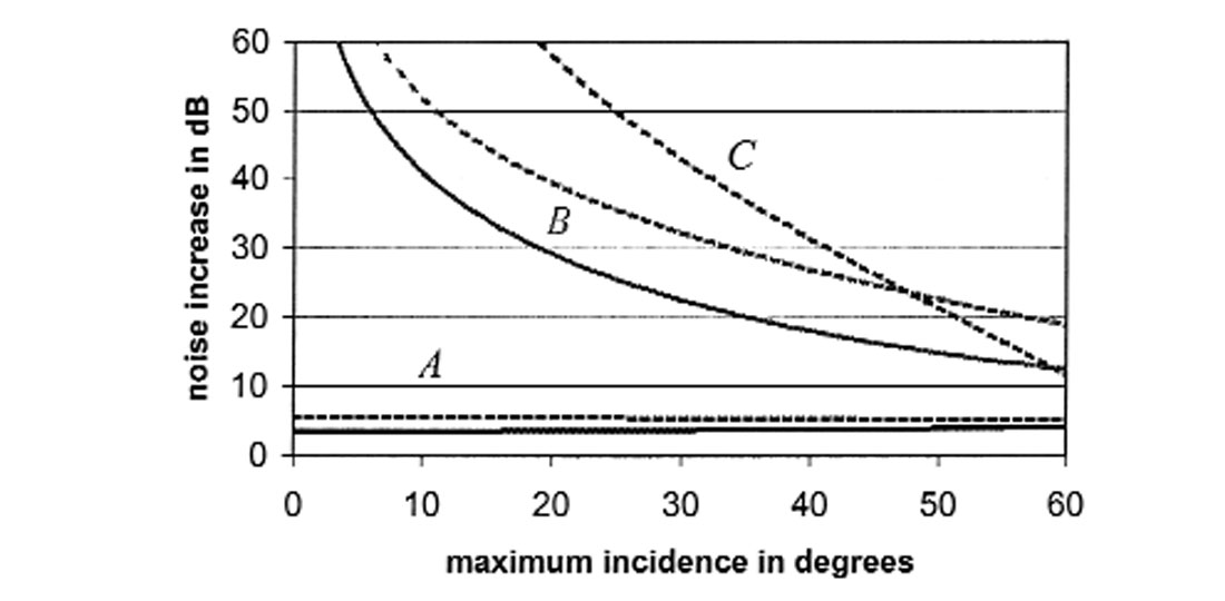
Figure 1 also shows the standard deviations for the three-term Shuey equation. The introduction of the third term C decreases the reliability of A (by 1.5 dB) and B (by 10 dB). At wide angles (approaching critical), the third term becomes more reliable than the second term because of the dramatic amplitude increase (the tangent square term “kicks in”).

Amplitude corrections

In the elastic theory, recorded amplitudes decay according to the spherical divergence of the wavefront. Compensating for this decay is fairly easy to achieve in a simple layered earth, but becomes a challenge in highly structured environments. True amplitude PSDM is then the most accurate tool. However, the subsurface is not purely elastic and the effects of attenuation should never be neglected (Smith and Gidlow, 1987). Q-compensation is now routinely performed, but the resulting prestack amplitudes are not fully satisfactory. It is therefore not uncommon, particularly for land data, to resort to statistical time and offset amplitude balancing. Time- and offset-dependent weights, derived on a survey-wide basis, and applied to the prestack gathers, are often considered proper AVO processing.

This deceptively mundane task has a dramatic effect on AVO results: It is a major factor in inflated gradient amplitudes and intercept leakage (Castagna and Smith, 1994; Cambois, 2000b). An average amplitude variation with offset is expected from Shuey’s equation. This behavior should be modeled and used as a reference for the statistical amplitude balancing. Alternatively, this problem can be totally avoided using the elastic impedance approach. Since the data are calibrated to well logs prestack, average amplitude variations with offset are automatically taken into account. This considerably reduces the burden of amplitude corrections, to the point where, in extreme cases, a long-window AGC should not necessarily be ruled out of proper AVO processing.

Wavelet variations

The wavelet shape can vary with time, space and offset. In a preserved amplitude sequence, the time variations can be handled with a deterministic Q-compensation. However, AVO studies are generally carried out over time windows short enough to guarantee stationarity. Spatial variations are taken care of with surface-consistent processes (e.g. Cambois and Magesan, 1997). The main problems are associated with offset variations, which can largely be attributed to NMO-stretching (source and receiver patterns and ghost directivity have a lesser impact). NMO-stretching acts like a low-pass, mixed-phase, non-stationary filter, of which the effects are virtually impossible to correctly remove (remember that Shuey’s model implicitly assumes a constant wavelet). As a consequence, it is often recommended to pick the reflection of interest prior to NMO-corrections and flatten it for AVO analysis. This avoids NMO-stretching but is only applicable where the target is an isolated reflection not affected by interference and tuning.

Again, this problem becomes a non-issue for elastic impedance. NMO-stretching effects are roughly angle-dependent so the wavelet can be assumed stationary in a limited-angle corridor. Each angle sub-volume (corridor stack) is then matched to its associated synthetic seismogram, which effectively removes the wavelet variations with angle. Note, however, that to be comparable the inverted sub-volumes must have similar bandwidth. This means that the far-angle resolution (the lowest) controls the resolution of the final result. This drawback does not seem to affect the standard AVO approach, but this is deceptive: The identical resolution obtained for all AVO attributes is only a consequence of intercept leakage and is therefore artificial.

NMO corrections

The Shuey model requires a perfect alignment of the prestack samples. Departure from this model introduces severe intercept leakage in the gradient and all other AVO attributes (Cambois, 2000b). Misalignments are primarily due to inaccuracies in the velocity field, themselves due to bad picks, poor interpolation of manual picks, or a combination of both. Obviously, the best effort has to be made at velocity picking, but dense picking (Adler, 1999) and rigorous QC (Le Meur and Magneron, 2000) should be generalized. Special care must also be taken in the presence of Class 2 AVO anomalies (Ratcliffe and Adler, 2000). Other possible sources of misalignment include long-wavelength statics (land), wide-angle residual NMO (often associated with anisotropy, see below) and non-hyperbolic reflections (in which case, PSDM is the only solution).

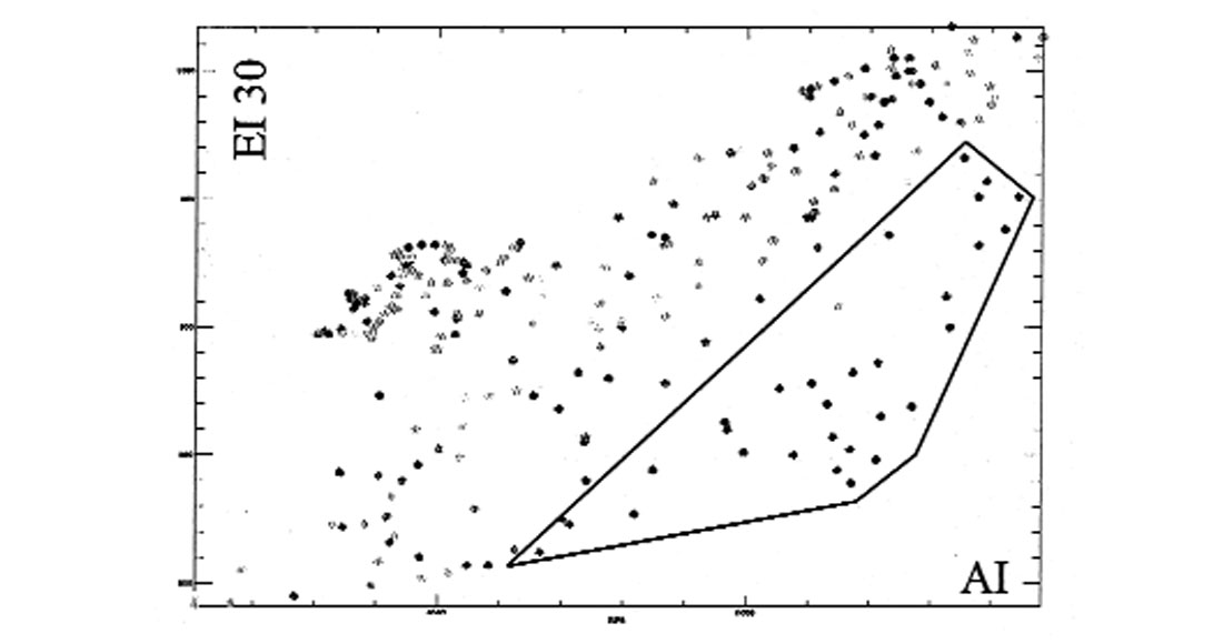
Elastic impedance is also sensitive to misalignments, albeit in a different way. Time differences between near and far angles do not generate any leakage but can still bias the results. Figure 2 shows an AI-EI crossplot derived from a well in West Africa. The reservoir sands are clearly identifiable. Figure 3 shows the same crossplot but after a 2 ms time shift between AI and EI: The sands cannot be detected. The maximum “tolerable” delay before the crossplot breaks down is a function of reservoir thickness (very thin in this case). However, this analysis should always be carried out as part of the feasibility study before venturing into any AVO project. Note that a layer-based stratigraphic inversion (Gluck et al., 1997) can in some circumstances identify minor time differences between the various angle cubes. The layers can then be reconciled before crossplotting.

Multiple attenuation

If multiples clearly represent a major departure from Shuey’s model, some multiple attenuation methods can be almost as harmful. A signal-preserving high-resolution Radon method has to be used (Herrmann et al., 2000). However, residual multiple energy can still be a major problem for AVO and elastic impedance, especially in cases of small moveout discrimination.

Anisotropy

At large offsets, seismic reflections in CDP gathers have a tendency to “curl up.” This phenomenon can be due to transverse isotropy or to the inaccuracy of the simple NMO equation at these offsets. Either way, a fourth-order term is needed to flatten these events and take full advantage of the wide aperture. (Picking this additional term is by no means a trivial task and requires specific training of the geophysicists and the auto-pickers.) The presence of anisotropy adds two major difficulties: The AVO equation changes (Thomsen, 1993) and the incidence aperture is reduced (Hilterman et al., 2000). These two effects combine for the worse: More parameters to estimate with less independent data.

Provided that the effects of anisotropy are mild enough to be neglected, it is tempting to use the increased aperture to estimate the three Shuey terms. Sufficient aperture and exceptional signal-to-noise ratio (Figure 1) may lead to reliable estimates of density contrasts. However, wide-angle data bring about new specific problems, from acquisition (array responses and source directivity become significant) to processing (the parabolic assumption for multiples no longer holds). There is definitely valid information at large offsets, but its quantitative use is still a work in progress.

Conclusions

In its simplest form, AVO analysis can be seen as the comparison between near and far angle reflections. If the comparison is purely visual (i.e. qualitative) the processing requirements are much less stringent than previously thought. For quantitative analysis, differencing of near and far angles is required and greater care must be taken during processing. However, the elastic impedance approach is a lot more forgiving than standard AVO: The only hurdles to be cleared are NMO corrections (near and far angle reflections have to be in phase) and residual multiple energy. As a consequence, elastic impedance makes AVO inversion accessible to the common man: No need for Hercules!