AVO projected pilot trace for dynamic trim statics

Abstract

P-wave fracture analysis provides a means to extract information about fracture density and orientation from a target reservoir. While successful application of any fracture analysis method requires that the technique be based on a sound theoretical framework, it turns out that careful handling of certain practical issues is also crucially important. Computation of dynamic trim statics, which are typically applied to measure residual moveout and also to flatten the seismic gathers prior to fracture analysis, is one such issue. Experience has shown that the construction of pilot traces via simple stacking can lead to erroneous estimates of dynamic trim statics in the case where the event of interest exhibits class II AVO. In fact, in such a case, computation (and/or application) of dynamic trim statics may do more harm than good. To solve this problem, we present a new approach to forming pilot traces, the so-called “AVO projected pilot trace” and we demonstrate the technique via synthetic data testing.

Introduction

Much work has been done in seismic fracture analysis on P wave data (e.g. Lynn et al., 1996; Teng and Mavko, 1996; Li, 1999; Gray and Head, 2000; MacBeth and Lynn, 2001; Zheng and Gray, 2002; Chapman and Liu, 2004; Chi et al., 2004; Parney, 2004; Zheng et al., 2004). Typically, a fractured zone is mathematically simplified as a Horizontally Transverse Isotropic (HTI) layer, which implies all fractures are vertical and oriented in one direction. There are two categories of methods for fracture analysis. One detects the Amplitude Variation with offset and AZimuth (AVAZ), and another detects the Velocity Variation with AZimuth (VVAZ). We have experimented with both categories on synthetic and real datasets, and have achieved successful results (Wang et al., 2007). For AVAZ we use Rüger’s method (Rüger, 1998), and for VVAZ, use the δ inversion (Zheng, 2006) which is a horizon based, layer stripping method.

Obviously the use of a good algorithm is a must for good fracture analysis. However, there are also some practical issues which may degrade the quality of fracture analysis if they are not handled properly. One of these issues is dynamic trim statics. Dynamic trim statics are necessary for achieving reliable fracture information from P wave seismic data, while pilot traces are important for good trim statics.

Motivation

It is common practice to calculate dynamic trim statics on some key horizons to obtain the Residual MoveOut (RMO) for VVAZ, and also to apply those dynamic trim statics to flatten seismic gathers prior to AVAZ inversion. The trim statics are calculated by cross correlation between each individual trace in the gather and a pilot trace, and the correlation window is typically short in order to focus on a particular horizon. One obvious approach to forming the pilot trace is simply to stack traces within a CMP gather (using either a full or partial offset stack). However, a problem arises when the reflection shows a polarity reversal with increasing offset. Specifically, the trim statics computation may cause misalignment of the seismic event if the trace has a different polarity or phase from the pilot trace. In other words, the short window trim statics process may do more harm than good for class II AVO if a stacked trace is used as a pilot trace.

The static shift between two seismic traces is typically chosen to be the lag of maximum correlation associated with the Normalized Cross Correlation Function (NCCF) of these traces. In practice, one may choose to use the maximum of positive values or the maximum of absolute values of NCCF in choosing this lag. Using the maximum of positive values of NCCF (the most common approach), is robust (in particular, it can effectively avoid the well-documented problem of cycle skipping) but will suffer from the aforementioned misalignment problem in the presence of class II AVO. On the other hand, using the maximum of absolute values of NCCF may avoid this misalignment problem but it is less robust . Specifically, in the special case of an isolated noise-free class II AVO reflection, use of the maximum absolute value of NCCF will “handle” the flipped polarity of the two traces by lining up the relevant reflection and keeping the original polarities, and ultimately produce the correct statics estimate. However in real data, there are neighbouring events around the class II reflection within the correlation window. These neighbouring events are often not class II AVO (i.e., the polarities of these events do not change as offset increases) and to the degree that these neighbouring events dominate the NCCF computation, even using the maximum absolute values of NCCF will not produce the correct static estimate. In addition, this latter technique (i.e., using absolute value of NCCF) will show less robustness in the presence of noise relative to the former technique.

Figure 1 shows an NMO corrected gather with four events. These events simulate wave propagation in a layered medium in which the first and fourth layers are isotropic, the second and third layers exhibit HTI anisotropy (with the same fracture density and orientation), and all the above four layers lie atop an isotropic half space (Figure 1, left hand side). Anisotropic amplitudes were modeled using the Rüger equation and traveltimes were computed based on the azimuthally-dependent moveout equation of Tsvankin (1997). The first event (event A at 1470 ms), which is the reflection from the top of the uppermost fractured layer, shows class I AVO behaviour. The second event (event B at 1506 ms) simulates a reflection from the boundary between the two vertically fractured (i.e., anisotropic/HTI) units. It also demonstrates class I AVO- type behaviour. Event C, the reflection from the base of the lowermost vertically fractured unit, is located at 1522 ms. This event exhibits class II AVO behaviour, as evidenced by the polarity reversal at the offset of 1500 m. Note that the main lobe of event C is a peak at near offsets and changes to a trough at far offsets. Finally, there is a class IV event (event D) at 1564 ms emanating from the interface between the fourth (isotropic) layer and the infinite isotropic half space. Note the presence of anisotropy - induced RMO on events B, C and D that is more obvious at far offsets. We have displayed the associated stacked trace on the same figure. Because event C is class II AVO, it appears as a weak peak on the stacked trace and is shifted downward about 8 ms compared to the time of the peak at the near offset (red circle on the stack). It follows that the phase of event C as seen on the stack differs from the phase of event C as seen on the near offset traces of the gather.

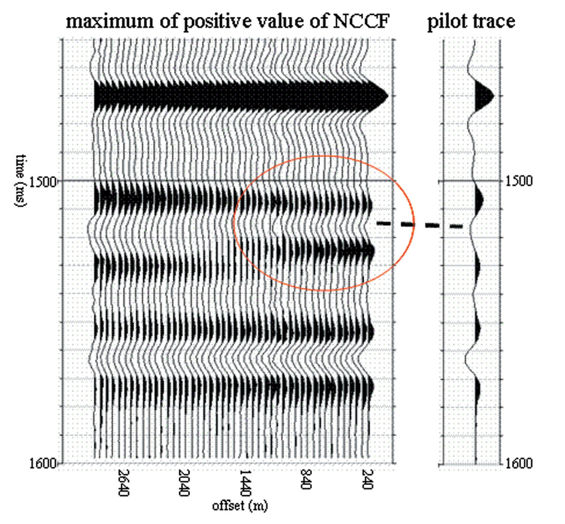
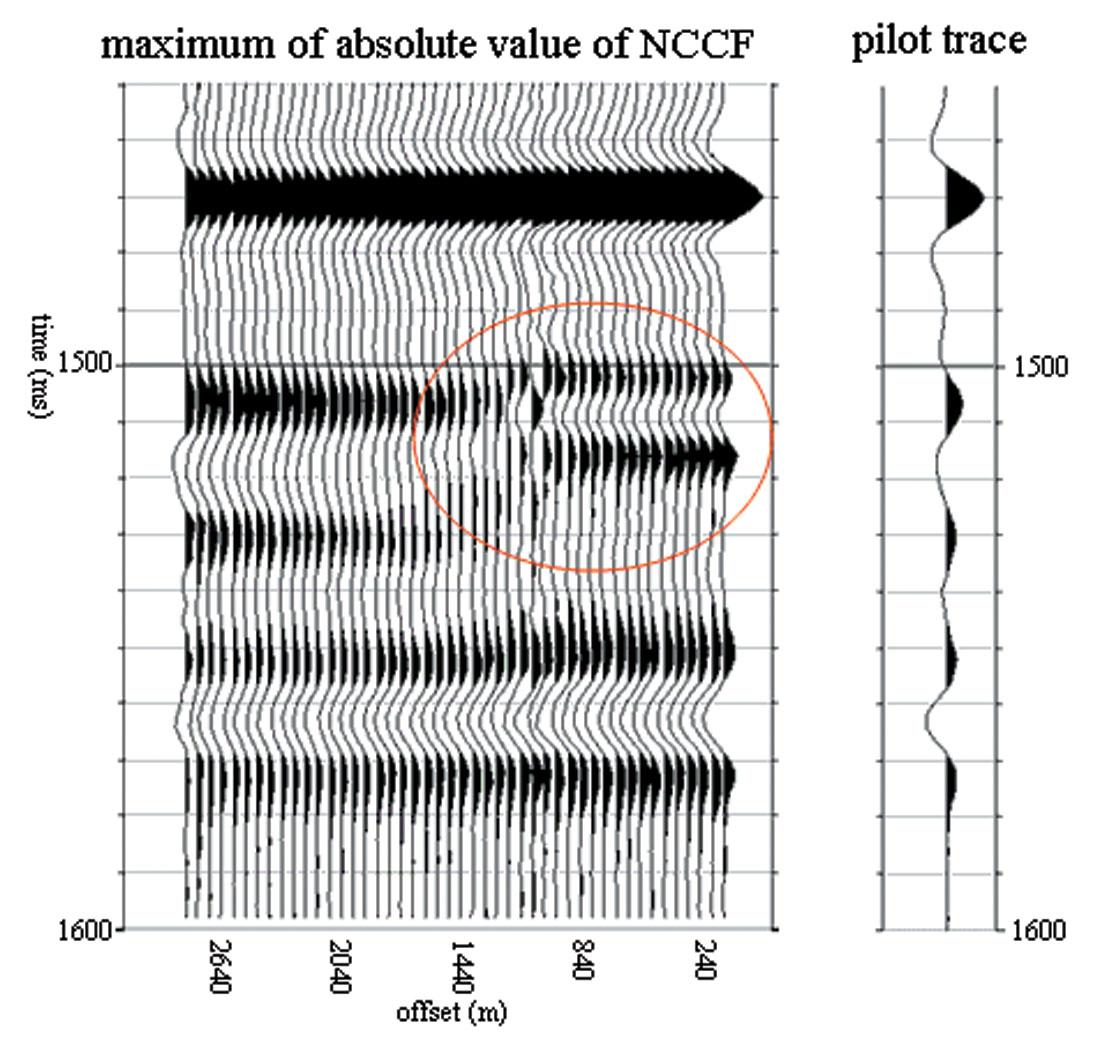
To demonstrate the potential problem, dynamic trim statics were calculated from the gather on Figure 1 using a stacked trace as a pilot trace. The dynamic trim static computation focused on three events, events A, C, and D, and the correlation window sizes were chosen to be 25 ms, 50 ms, and 25 ms, respectively. The dominant frequency of the seismic data is about 40 Hz. The maximum allowed static shift was limited to 8 ms, which is about one third of the period of the seismic wave. Figure 2 shows the gather after applying dynamic trim statics computed based on the maximum of positive values of NCCF and Figure 3 shows the gather after applying dynamic trim statics computed based on the maximum absolute values of NCCF. Both of them work very well for events A and D, but neither works for event C. In particular, both give erroneous static shfits at near offsets, as evidenced by the red circles on Figures 2 and 3. When the maximum of positive values of NCCF is used to determine the amount of static shift, the near offset traces were forced to shift downward (Figure 2) to line up the trough just below the event B (dashed line on Figure 2). When the maximum absolute values of NCCF is used, the near offset traces were shifted upward to line up the peak of event C of the near offset trace and the trough just below event B of the pilot trace (Figure 3). In this example, false statics were introduced by using the stacked trace as a pilot in either mode of implementation (i.e., using maximum of either absolute or positive values of NCCF). With this unexpected behaviour of the dynamic trim statics, there is no doubt the following fracture analysis will yield erroneous result. A better approach is needed to avoid this problem.

AVO projected pilot trace

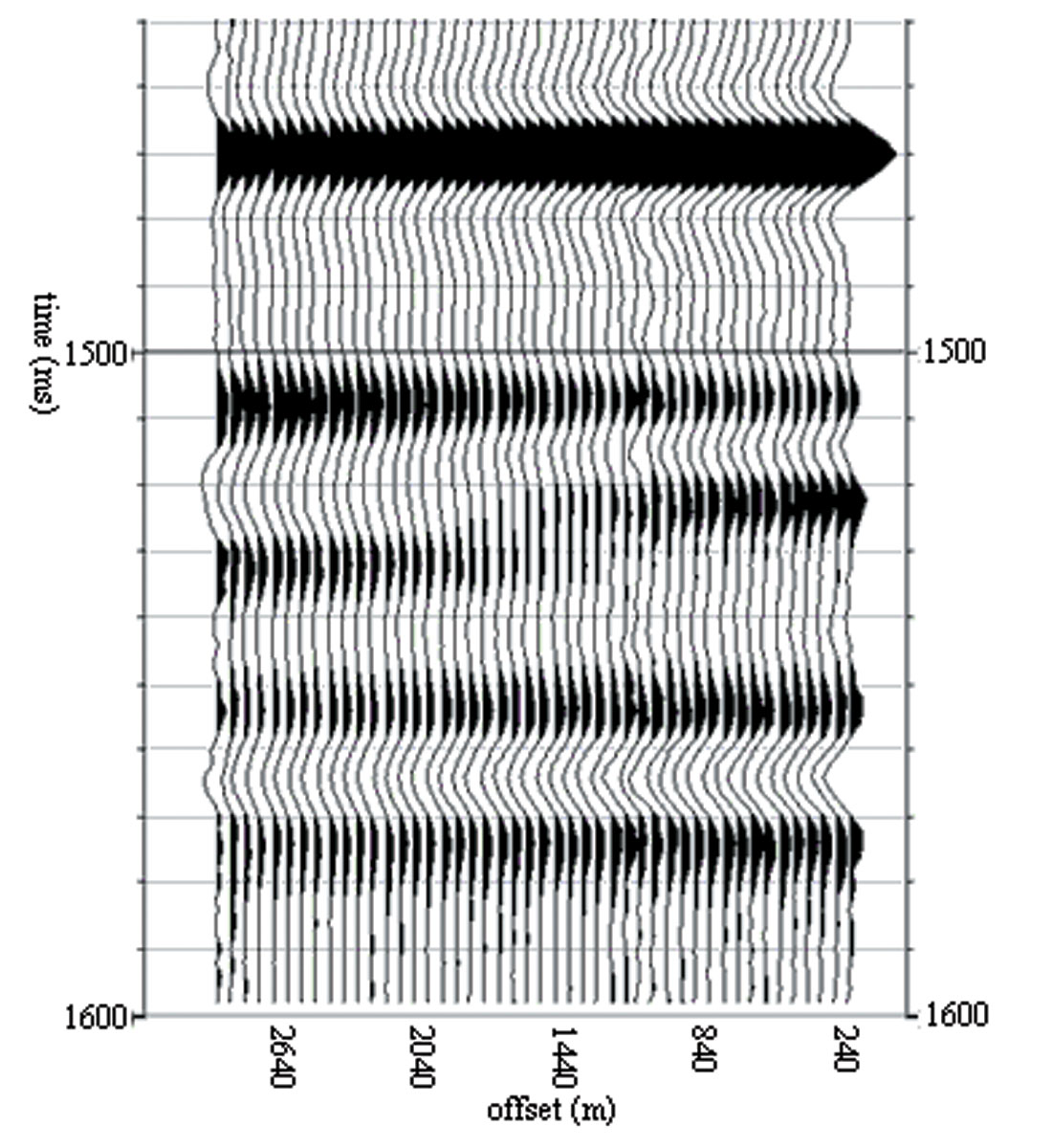
To solve the misalignment problem, we developed a new method for forming the pilot trace for correlation. We use the isotropic AVO intercept and gradient (Shuey, 1985) to project a pilot trace at the same offset as the trace to be correlated, thereby avoiding correlating two traces of different phase/polarity. In practice, we run AVO inversion first to extract the AVO intercept and gradient using the same gathers which are used for fracture analysis. Then, when we calculate the trim static for a trace (target trace), we generate a pilot trace on-the-fly by using the intercept and gradient, plus the offset of the target trace and the same velocity at the location based on Shuey’s equation. The fact that our pilot trace construction assumes an isotropic theory, while our data traces are presumed to exhibit HTI-type anisotrpoy does not seem to represent a serious inconsistency from the viewpoint of dynamic trim statics computation, presumably because the isotropic component of the amplitude gradient is typically larger than the anisotropic component, and therefore the pilot trace typically has the same phase/polarity as the target trace. Figure 4 shows the gather after applying dynamic trim statics using the AVO projected pilot trace. All events, including event C, are flat after applying dynamic trim statics. Clearly, this method has successfully avoided the trouble of polarity reversal or phase difference between the pilot trace and the gather.

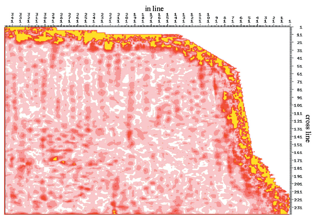
To further verify the advantage of the AVO projected pilot trace, we built a synthetic dataset based on a real survey geometry. The model is the same as that in the previous example, but the fractured layers only exist within a spatially localized circular area (50 CDP radius) centred at inline 200 and cross-line 105. Outside this circular area, all layers are isotropic. The anisotropic wave propagation effects (i.e. amplitude and traveltime behaviour) were modeled using the same approach described earlier in the text. We used both the stacked trace and the AVO projected trace as pilot traces followed by the δ inversion. The results of the δ inversion are shown on Figures 5 and 6. When AVO projected pilot trace is used, the VVAZ result matches the input model, and the circular anisotropic anomaly is properly resolved (Figure 5). However, when the stacked trace is used as the pilot trace, the δ inversion result is erroneous (Figure 6). In particular, “false” statics estimates have introduced false anisotropy throughout the survey.

Conclusions

The quality of fracture analysis largely depends on the data preparation. In the case of class II AVO, the phase and polarity on the stacked trace are different from those associated with each individual trace in the gather. One may therefore get incorrect RMO measurements by correlating the seismic gathers with a stacked trace as a pilot trace, in which can lead to erroneous fracture attribute estimates. The AVO projected pilot trace is formed by forward modeling using AVO intercept and gradient information derived from an upstream AVO inversion of the same seismic gather and using the same offset and velocity of the trace to be correlated. This approach avoids the misalignment problem caused by different phase/polarity of the pilot and the target trace. Synthetic testing shows the fracture anomaly can be properly resolved by using the AVO projected pilot trace for dynamic trim statics; by contrast, by using the stacked trace as a pilot, we obtain an erroneous characterization of the fracture regime.