Abstract
Azimuthal AVO analysis can be split into two parts: the Amplitude Versus Offset (AVO) analysis and the Amplitude Versus Azimuth (AVAz) analysis. For regularly sampled data in azimuth, the properties of the Fourier transform allow these problems to be treated separately. If we calculate a Fourier transform of the AVAz PP reflectivity data at a particular angle of incidence, we obtain Fourier Coefficients (FCs) that parsimoniously describe the AVAz and anisotropy. It is possible to attach physical significance to each of the FCs by assuming simple rock physics models that relate the anisotropy to the fractures. Assuming a single vertical fracture set, the second FC is approximately equivalent to the anisotropic gradient. Other FCs convey additional independent information about the fractures. The different FCs may be combined in a nonlinear fashion to estimate more fundamental fracture parameters including an unambiguous estimate of the symmetry axis. The FCs are calculated using a limited range of offsets or angles, which places less demands on the data acquisition. This may be advantageous for land 3D data sets, where near offsets are particularly under sampled.
Introduction
The P-wave AVAz reflectivity for a given angle of incidence may be described compactly in terms of a Fourier series (Ikelle, 1996; Sayers and Dean, 2001). Note that a Fourier series is a sum of weighted sinusoidal components which added together approximates a given function. We call the weights on the sinusoidal terms the Fourier Coefficients (FCs). These FCs may be calculated from the AVAz reflectivity using a Fourier Transform. Because of the orthogonality of the Fourier Transform, each of the FCs convey unique and independent information making them ideal attributes to interpret. Despite this, the use of FCs has yet to gain wide spread use. Perhaps one of the barriers to their acceptance is a lack of understanding of what they mean in terms of rock parameters and how they relate to more traditional methods.
This paper describes the physical significance of each of the azimuthal FCs for PP reflectivity data in terms of Linear Slip (L.S.) theory (Schoenberg, 1980), for the special case of a single vertical fracture set within a background isotropic rock. Under this assumption, the FCs can be related to the near offset Rüger equation (2002). It is therefore possible to use FCs to estimate the anisotropic gradient using only the far angle (offset) data. Also, the 2nd and 4th FCs can be used to resolve the symmetry axis azimuth ambiguity inherent in the near offset Rüger equation if we assume that the cracks are “penny shaped”.
We begin by reviewing some of the key attributes generated by the near offset Rüger equation and some of this equation’s limitations. One of the goals of our paper is to show how these attributes may be reproduced using FCs and how some of the limitations are overcome. The next section introduces the azimuthal FCs by way of a simple example. The example is used to illustrate the general behaviour of the FCs and how they may be calculated in practise. We then show that the FCs arise naturally out of a reparameterization of the Pšenčik and Martins (2001) linearized PP reflectivity expression for arbitrary anisotropy. Linear Slip theory is then quickly reviewed under the assumption of a single vertical fracture set with the goal of providing a framework to relate the FCs to fracture parameters. The parameters Bani and κ are introduced as functions of L.S. parameters and shown to be, to a linear approximation, scaled versions of the magnitude of the 2nd and 4th FCs. These relationships are used as a means to interpret the FCs and compare the FC approach with that of the near offset Rüger equation.
This comparison is illustrated on a dataset from West Central Alberta for which we have image log data. Hunt et al. (2010) have previously studied this dataset. They compared various fracture predicting attributes including the anisotropic gradient generated from the near offset Rüger equation, most positive curvature, and the fractional change in azimuthal velocity. These attributes were compared quantitatively to the image log data from two horizontal wells. Correlation coefficients were generated between the attributes and the image log data and between the different attributes. This work extends the previous work by including the azimuthal FC attributes in the analysis. The FCs calculated from large angle data produced higher correlation coefficients with the image log data than the attributes generated from the near offset Rüger equation. One advantage is that the FCs can be generated using just the mid to large offset seismic data, thereby bypassing some of the sampling issues inherent in land 3D seismic acquisition. The paper lastly discusses how it is possible to use several of the FCs in combination to estimate fracture weakness parameters and resolve the symmetry axis ambiguity.
Rüger equation
The azimuthal reflectivity of media with HTI anisotropy and the same symmetry axes is described by the near offset Rüger equation (Rüger, 2002)

where ϕ represents the source to receiver azimuth, θ is the average angle of incidence, A is the intercept, Biso is the isotropic gradient, Bani is the anisotropic gradient and ϕsym is the azimuth of the symmetry axis. Hudson (1981) theory may be used to show that the anisotropic gradient Bani is proportional to the crack density. The symmetry axis is perpendicular to the strike of the fractures. This near offset approximation ignores higher angle terms, introducing a bias into the Bani estimate. The advantage of using this approximation is that equation (1) may be linearized by rewriting it in terms of cos(2ϕ) and sin(2ϕ) and thus be solved in a straightforward fashion using least squares inversion (Downton and Gray, 2006). The disadvantage of this approximation is that it is impossible to tell whether the anisotropic gradient is positive or negative, thus introducing a 90 degree ambiguity into the estimate of ϕsym.
Azimuthal Fourier Coefficients
To introduce the concept of azimuthal Fourier coefficients a simple P-wave reflectivity model was generated for an isotropic layer over an anisotropic layer (Figure 1). The second layer’s anisotropy is due to a single vertical fracture set. The actual parameters are not all that important. What is important is the observation that the amplitude versus azimuth reflectivity can be described using a Fourier series. The model’s average AVO is shown in Figure 1a whereas the remaining panels show the azimuthal reflectivity at various angles of incidence. The azimuthal reflectivity is the sum of the sine and cosine functions or, more equivalently, a Fourier series. The solid curve shows the continuously sampled function while the stars show the reflectivity sampled every 22.5 degrees. In practice the data is only recorded at some finite number of locations, which impacts our ability to estimate the FCs.
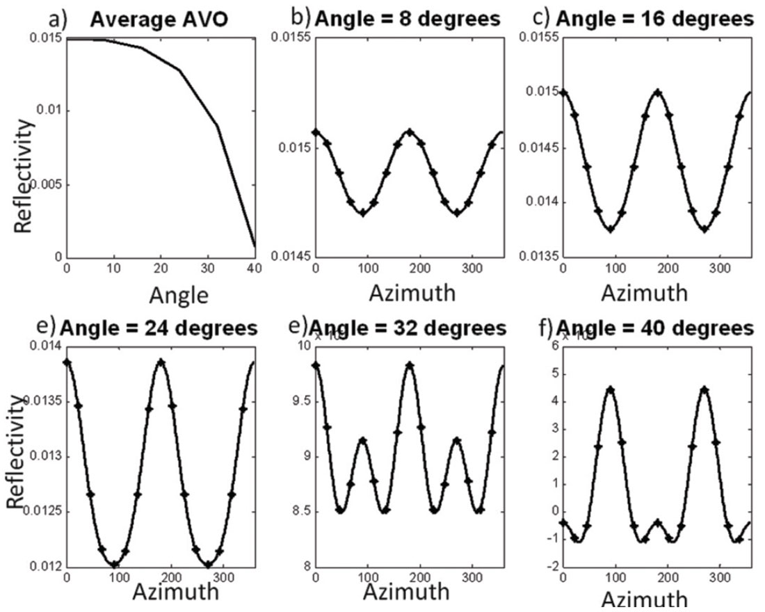
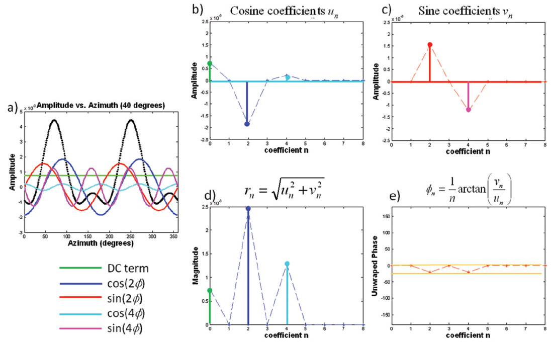
Figure 2 shows the result of decomposing the 40 degree incidence angle AVAz PP reflectivity into its constituent sine and cosine functions represented by the Fourier series
The green line in Figure 2a is the D.C. component, which is the average amplitude at an incidence angle of 40 degrees. The blue and red curves represent the cos(2ϕ) and sin(2ϕ) components, while the cyan and magenta curves represent the cos(4ϕ) and sin(4ϕ) components. All of these functions sum together to give the azimuthal reflectivity. Figure 2b and 2c plot the amplitude of the different cosine and sine functions in a similar color scheme. In practice these coefficients are calculated using a Discrete Fourier Transform (DFT). For the case of N regularly sampled data, the cosine coefficients un are calculated using
while the sine coefficients vn are calculated using
for integer values of n such that n ≥ 0. Alternatively, the Fourier series can be written in terms of magnitude (Figure 2)

and phase (Figure 2e)
This later formulation is perhaps more intuitive since the phase can be related to the azimuth of the fractures. The Fourier series for the magnitude and phase parameterization is
Note that in Figure 2 only the even FCs have nonzero values. This is a general result for PP data due to reciprocity. The other interesting thing to note about Figure 2 is that the maximum nonzero Fourier coefficient is n=4. This is a consequence of using a linearized approximation to calculate the reflectivity (Appendix A). Sayers and Dean (2001) reported seeing some energy on the 6th Fourier coefficient using nonlinear modeling. Since the energy of the 6th FC is much smaller than the energy of the 4th coefficient in practice we need only estimate the n=0, 2 and 4 FCs.
The workflow to calculate the azimuthal FCs on real data depends on the seismic data acquisition geometry and the type of prestack migration performed prior to the analysis. The simplest case for the purposes of this analysis is to perform migration and output the data regularly as a function of azimuth. An azimuthally sectored migration outputs the data in such a fashion. Assuming this is the case, then within each angle sector the data must be mapped from offset to angle of incidence, outputting the data in a regular fashion. Then, for each angle of incidence, the FCs are calculated using equations (3) and (4) in a similar fashion as the previous example. Care must be taken to adequately sample the data so that the Nyquist criterion is met. In order to estimate the n=4 FC the data must be sampled no coarser than 22.5 degrees.
For the more complex case of irregularly sampled data in azimuth, a least squares inversion may be performed using the DFT as the linear operator. This is the case for common offset vector (COV) migrated data. For COV data there is also the extra complexity of AVO / AVAz cross-talk (see Appendix A).
If a least squares inversion is performed, then the fact that the n=1 and n=3 FCs are zero may be used to reduce the number of azimuths needed for the analysis. To accurately estimate the n=4 FC in the presence of noise the minimum azimuthal sampling is 30 degrees.
Azimuthal FCs for arbitrary anisotropy
The Fourier Coefficients can be derived for arbitrary anisotropic media by rearranging the linearized P-wave AVAz equation (1) of Pšenčik and Martins (2001) in terms of sine and cosine functions resulting in the truncated Fourier series (Appendix A)
where
where the wij coefficients are defined in Appendix B. Without going into the exact details of the expressions for the coefficients there are several observations that can be made. For the most general case, that of arbitrary anisotropy, there are only 5 nonzero coefficients. The n=0 FC is the classic 3 term AVO expression where the definitions of A, B and C are modified by the anisotropy. The n=4 FCs are angle dependent functions of a single variable. The n=2 FCs have the most complex form, being a function of two variables. The implication of this is that the phase of the 2nd FC can change as a function of the angle of incidence.
In order to gain an intuitive understanding of what each FC means we next introduce a rock physics model linking the elastic properties to the fracture properties. Furthermore, in order to compare these results to the Rüger equation it is assumed that the anisotropy is due to a single vertical fracture set.
Linear slip theory
Linear Slip theory (Schoenberg, 1980) may be used to relate elastic parameters to fracture parameters. This theory models fractures as a perturbation from the background compliance of a non-fractured rock, which we assume to be isotropic. The total compliance of the rock S is the sum of the background compliance Sb plus the compliance due to the fractures Sf. The fractures can be modeled as an imperfectly bonded interface where the traction is continuous but the displacement might be discontinuous. The displacement discontinuity is linearly related to the traction, and in its simplest form, the fractures normal to the x-axis give rise to HTI anisotropy (Schoenberg and Sayers, 1995). For example, the displacement discontinuity normal to the fracture is proportional to the normal stress. This proportionality constant is the normal fracture compliance BN. Similarly, the tangential fracture compliance BT may be defined. Instead of working with compliances, we choose to parameterize the problem in terms of the normal weakness parameter

and tangential weakness parameter

where M=λ+2μ. These are fractional parameters which range from 0 to 1. In both cases, when the fracture weakness is zero the fracture has no influence on the compliance. The normal weakness is also sensitive to fluid fill within the crack, since the fluid makes the crack less compliant. Bakulin (2000) shows that the anisotropic gradient may be written in terms of these weakness parameters so that

where χ=1-2g and g is the square of the S-wave to P-wave velocity ratio of the non-fractured rock. The difference operator Δ represents the difference in layer properties between the lower and upper media, thus ΔδT is the difference in tangential weakness between the two layers. For future reference the variable

is also introduced. Both κ and Bani are weighted differences of the tangential and normal weaknesses with slightly different weighting factors.
Azimuthal FCs for a single vertical fracture set
For the case of a single vertical fracture set parameterized in terms of κ and Bani equation (8) reduces to
where

and

As in the case of general anisotropy the D.C. component (n = 0) is the 3-term AVO expression where the definitions of A, B, C are defined in Appendix C. The terms are the same as in the isotropic case but with the addition of fracture weakness terms to account for the extra compliance introduced by the fractures.
For the case of data that is regularly sampled in azimuth, the different FCs are independent; thus it is possible to isolate the D.C. component and solve separately for the A, B and C parameters. However, converting these parameters to fracture weakness, density, P-wave, and S-wave Impedances estimates is an underdetermined problem. If the fracture weakness parameters are ignored then the resulting interpretation of the isotropic parameters is biased. One possible solution is to first solve for the fracture parameters using the nonzero FCs.
For small angles of incidence, the n = 2 FC is, to a linear approximation, an angle scaled version of the anisotropic gradient. This can be written mathematically as

The implication of equation (21) is that the anisotropic gradient can be calculated by scaling the magnitude of the 2nd FC so

For example, one could generate an estimate of the anisotropic gradient by calculating the 2nd FC over a limited range of angles centered around 30 degrees and then multiply the result by 8. Only mid to far offsets are needed in this calculation. In contrast, inversions using the near offset Rüger equation use all the offsets in the calculation. Good azimuthal sampling of the near offsets is typically problematic, particularly on land 3D surveys. Both the near offset Rüger equation and equation (21) make the same linear approximation, which is that the sin2(θ)tan2(θ) terms are ignored. Figure 5 shows a comparison of the anisotropic gradient calculated both ways and will be discussed in greater detail in a later section.
The uncertainty of the anisotropic gradient is inversely proportional to sin2(θ). The uncertainty gets larger as the angle of incidence gets smaller, and with typical noise levels the estimate becomes unstable for angles less than 25 degrees. From equation (18) it is evident the phase is the azimuth of the symmetry axis. For the 2nd FC, the phase wraps every 90 degrees and so has the same ambiguity issues as the near offset Rüger equation.
The 4th FC is a scaled version of κ, so similar to above, κ may be estimated by multiplying the 4th FC appropriately, which can be written as

Nordegg Example
One of the issues in working with fracture estimates is validating the results. To calibrate our estimates we chose to perform this analysis on a dataset from Western Canada with image log control data. Hunt et al. (2010) described this dataset and analyzed it in great detail. One advantage to using this dataset was that other fracture predicting attributes, including the near offset Rüger equation, were run on it and available for comparison.
The 3D seismic dataset we used is roughly 600 square kilometres in area with a nominal source and receiver line spacing of 600 m. This results in nominally 27 fold data. Both the fold and line spacing are suboptimal for the purposes of performing a prestack azimuthal analysis. The data was 5D interpolated to improve the sampling, and then prestack migrated. Downton et al. (2010) showed that the use of 5D interpolation followed by migration improved the correlation between the image log data and the anisotropic gradient generated from the near offset Rüger equation. These same gathers are also used in this study.
The formation of interest for this study is the naturally fractured Nordegg Formation. In this area, the Nordegg is a gas charged sublithic sandstone at a depth of about 3300 m. The reservoir is about 12 m thick with permeability’s between 0.01 to 0.1 mD. The 6% matrix porosity is thought to be augmented by the areas complex system of faults and fractures. The available image log data suggests that the fractures are near vertical with one dominant azimuth controlled by the principal stress in the area. Thus, the image log data suggests that the fractures are consistent with our assumption of a single vertical fracture set.
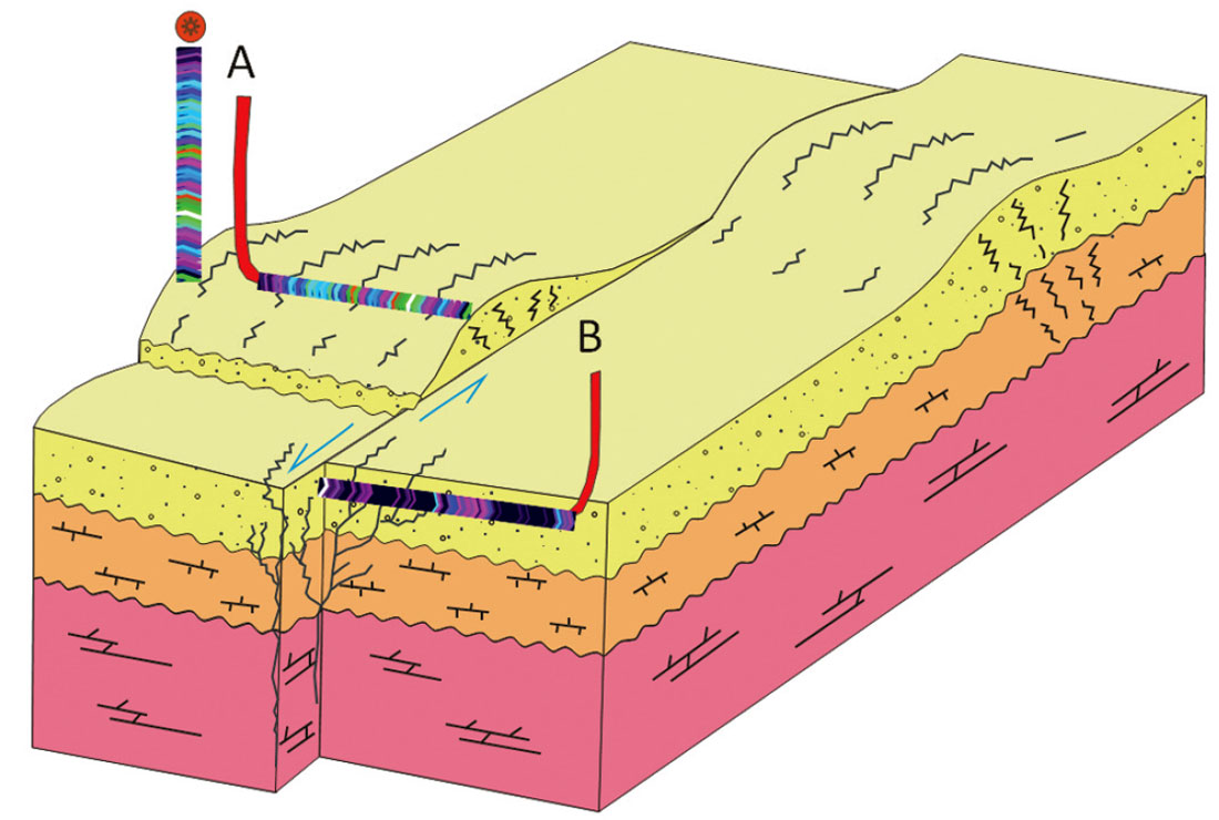
There are two horizontal wells and one vertical well with image log data in the study area (Figure 3). Horizontal Well A was drilled along the crest of the anticline and encountered significant fracturing. Well B was drilled into a strike slip feature and encountered fewer fractures. Lastly, there is a vertical well encountering fractures at the Nordegg level. The image log data from these wells were used to quantify the ability of each attribute to predict fractures by calculating the correlation between the three wells and each of the attributes.
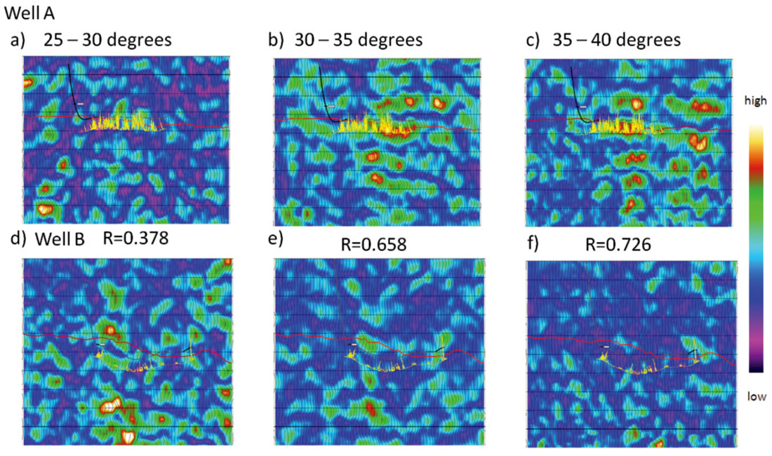
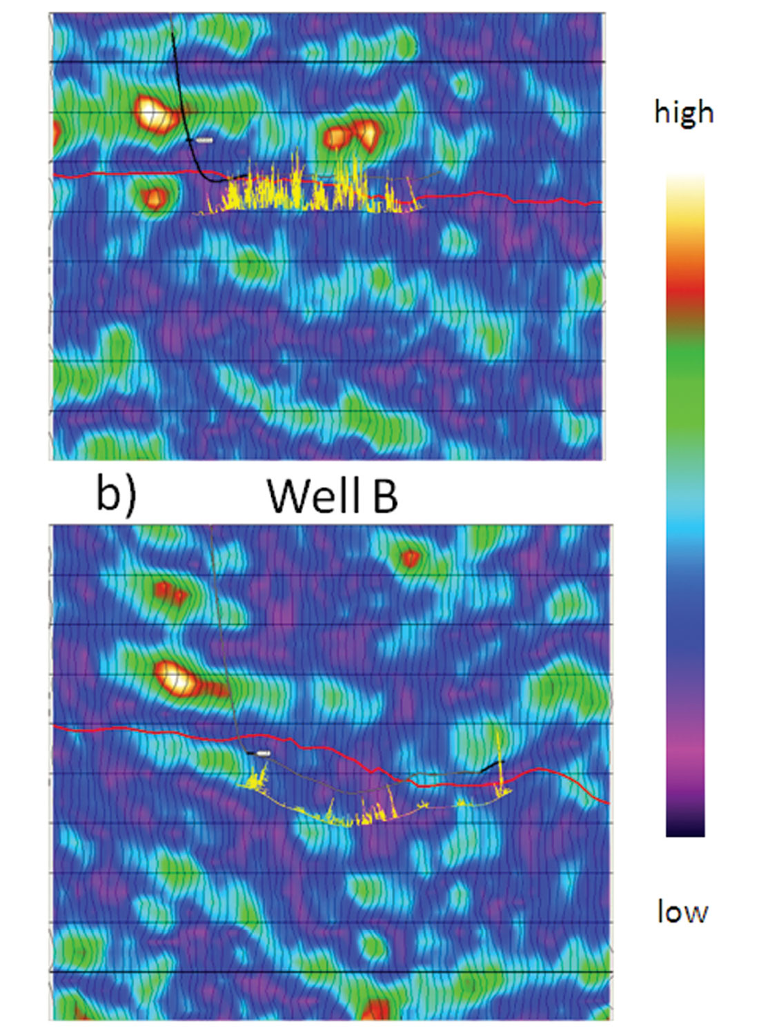
The anisotropic gradient was calculated from the magnitude of the 2nd FC based on three different angle ranges: from 25 degrees to 30 degrees, from 30 to 35 degrees, and lastly from 35 to 40 degrees, and then compared to the well control (Figure 4). The interpreted Nordegg horizon is show in red, while the well trajectory is shown in black. The fracture density calculated from the image log is shown as a yellow curve with the vertical excursion proportional to the fracture density. In each case the scaled 2nd FC predicts more fractures at well A than well B, which is consistent with the well control. The analysis at smaller angles seems to be considerably noisier than the large angles. In order to quantify the quality of the fit, the correlation coefficient R was calculated between each attribute volume and the image log data. The correlation increases with the angle of incidence used in calculating the FCs. This could be either consequence of the uncertainty decreasing with the larger angles or evidence of the nonlinearity of the 2nd FC manifesting itself.
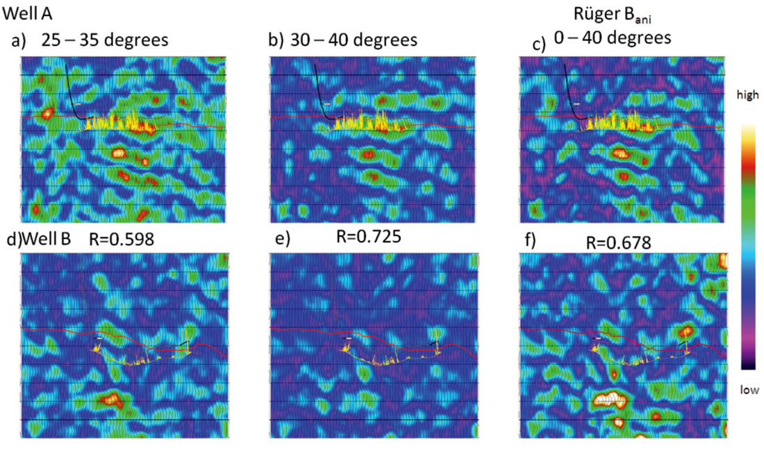
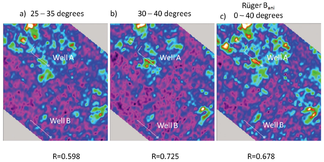
The angle scaled 2nd FC was also calculated using a 10 degree angle range (Figure 5). Ideally one wants to calculate the FCs over as narrow an angle range as possible to minimize the crosstalk between the AVO and AVAz (Appendix A). However, this desire must be tempered by the requirement that there is adequate fold to perform the analysis. In Figure 5, the 2nd Fourier coefficient was calculated over angles from 25 to 35 degrees, and from 30 to 40 degrees. Figure 6 shows the same information but as horizon slices. Once again the correlation coefficient increases with larger angles of incidence. For comparison the anisotropic gradient generated by the near offset Rüger equation is also shown. This was calculated using angles from 0 to 40 degrees, with the larger angles contributing most of the response. Somewhat surprisingly, the near offset Rüger inversion has a lower correlation coefficient than the result from the angle normalized 2nd FC calculated from 30 to 40 degrees. It was our expectation that the Rüger inversion would have a higher correlation due to its better signal-to-noise characteristics, since it was calculated using more data and higher fold. The fact that it does not suggests that the improvement in the correlation coefficient is most likely due to the nonlinearity of equation (19).
Goodway et al. (2006) showed that the anisotropic gradient in certain situations can be zero even if the fracture weakness parameters are nonzero. This is a result of the fact that the anisotropic gradient is a weighted difference of the fracture weakness parameters ΔδT and ΔδN (equation 16). The linearized magnitude of the 2nd FC (equation 21) behaves in a like manner. However, the magnitude of the nonlinear 2nd FC (equation 19) written in terms of weakness parameters
has the ability to resolve this issue. If at one angle of incidence the nonzero fracture parameters are summing to zero, then the analysis can be performed at another angle with different weights and results. By looking at the magnitude at two angles of incidence, one can ensure that this situation never occurs. Certain combinations of weights (angles) should more optimally convey the fracture information. It would be better to directly invert for the fracture parameters and thus avoid this issue. The fact that the relative weighting between ΔδT and ΔδN changes as a function of angle may be exploited to directly invert for these fracture properties. This is explored in the last section of this paper.
The 4th coefficient was used to calculate κ (Figure 7). The resulting correlation coefficient of 0.477 between the image log data and κ was not as good as the 2nd FC (Table 1). At well B both the 2nd and 4th coefficients give similar interpretations. However, at well A the κ anomaly appears to be above the Nordegg Formation resulting in a poorer correlation. This might be due to rock physics: κ might not be as good a fracture predictor as Bani in this case. Since κ is also a weighted difference of ΔδT and ΔδN with slightly different weighting terms it is therefore more likely the inferior results are a result of inadequate fold and signal-to-noise considerations. Recall that the original fold of this dataset prior to interpolation was 27 and there needs to be a least 6 distinct azimuths over a narrow angle range in order to predict the 4th FC. This dataset was chosen because of the availability of the image log data but we had some concerns about the fold of the data going into the analysis.
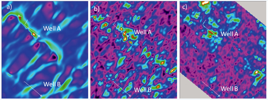
There have been a number of other fracture predicting attributes generated in the past on this dataset, including most-positive curvature and fractional azimuthal velocity analysis. The physical basis for these attributes are different but they share in common the fact they all are responding to fractures, thus there should be some similarity. Figure 8 shows a comparison of these attributes and the 2nd FC. Correlation coefficients were generated between all these attributes and the image log data and summarized in Table 1. Interestingly, the anisotropic gradient calculated from the 2nd FC from 30 to 40 degrees has a higher correlation to the other attributes than the result from the Rüger equation.
| Upscaled Fracture Density | Most-Positive Curvature | VVAz | |
|---|---|---|---|
| Table 1. The correlation coefficients generated between the image log data and the various seismic attributes. Note the magnitude of the 2nd FC has the highest correlation to the image log data and the other seismic attributes. | |||
| Upscaled Fracture Density | 1.000 | ||
| Most Positive Curvature | .613 | 1.000 | |
| Azimuthal Velocity (VVAz) | .498 | .445 | 1.000 |
| R2 (25 - 35 degrees) | .598 | .710 | .476 |
| R2 (30 - 40 degrees) | .725 | .734 | .541 |
| Rüger Bani | .678 | .677 | .509 |
| R4κ (all angles) | .477 | .424 | .325 |
Other Parameterizations
Both the 2nd FC (equation 24) and the 4th FC (equations 17 and 20) are weighted sums of the fracture weakness parameters ΔδT and ΔδN. It is thus possible to solve for these parameters explicitly, but the problem is nonlinear. If one considers only the information coming from the 2nd FC there are two distinct solutions which are a result of the phase wrapping associated with the n=2 FC. Including the information from 4th coefficient resolves this problem and the azimuth ambiguity inherent in the Rüger equation. The reformulation into ΔδT and ΔδN results in a set of equations which are consistent with Shaw and Sen (2006). This mapping from Bani and κ to ΔδT and ΔδN also provides a link to the layer parameters δN and δT estimated by the azimuthal inversion of Downton and Roure (2010).
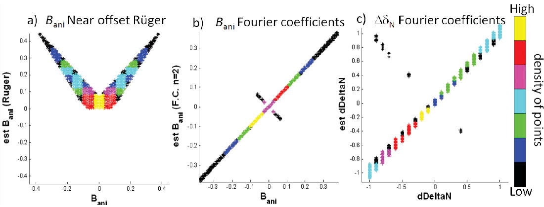
Figure 9 shows the results of performing a nonlinear inversion for ΔδT and ΔδN on synthetic data. The misfit function is multi-modal as this is a nonlinear problem. In order to verify that the nonlinear inversion correctly estimates the global misfit minimum, a large number of models were tested (> 16,000). Different combinations of the symmetry axis, normal and tangential weaknesses were used to generate forward models using the Zoeppritz equation. Noise was added to create a signal-to-noise ratio of 10:1. The resulting synthetic data were then inverted for the isotropy plane ϕiso, ΔδN and ΔδT. Bani and κ were also calculated from ΔδN and ΔδT . Figure 9 shows the estimated variables compared to the actual variables. If the estimated value corresponds to the ideal value the points should be on the diagonal line connecting the lower hand left corner to the upper right hand corner. The figures are color coded so that the color represents the number of solutions that fall within a particular bin. The nonlinear inversion properly assigns the correct sign to Bani in 99.5% of the models (Figure 9b). In the case when κ = 0 (a small percentage of the models) the n = 4 FC is non-informative and there is not enough information to uniquely determine the symmetry axis. This contrasts with the near offset Rüger equation (Figure 9a) where the solution for Bani is multi-modal. In Figure 9a the positive solution is chosen and displayed. Small Bani values estimated by the Rüger equation show significant bias due to the higher offset term being neglected. In the case of nonlinear inversion, there is little error in the azimuthal estimate other than the points associated with κ = 0. The normal and tangential weakness estimates plot along the diagonal again showing the estimated values accurately predict the majority of cases. Only the normal weakness is shown in Figure 9c but the tangential weakness behaves in a similar fashion. The transformation amplifies the random noise so there is more dispersion in the estimates of ΔδN and ΔδT than Bani and κ. The inversion relies on information from the sin2 θ and sin2 θ tan2 θ AVO basis functions so large angles are needed to get reliable results.
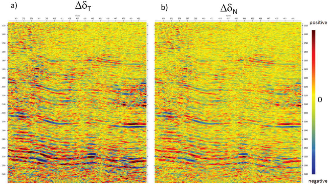
The nonlinear inversion was tested on a real seismic dataset. Profiles of the ΔδN and ΔδT estimates are shown in Figure 10. The estimate of the azimuth of the symmetry axis is compared with that of the near offset Rüger equation in Figure 11. The phase ambiguity (wrapping) is clearly evident in the Rüger result. The circled area in Figure 11 shows the phase quickly changing from -50 degrees to 40 degrees at a layer boundary. The result from the nonlinear inversion is more consistent across the boundary. Furthermore, the result seems to be consistent with the principal stress field in the area. Note the phase can only be estimated when the weakness parameters are nonzero. Since the weakness parameter estimates are band limited this makes the phase estimates look noisy. At this point in time, these results are non-calibrated and more work needs to be done to understand the stability of the nonlinear inversion.

Discussion
The assumption of a single vertical fracture set used in this paper is made to aid in the comparison to more traditional methods (i.e. the near offset Rüger equation). However, it should be noted the FC method generalizes to more complex forms of anisotropy. For example, Sayers and Dean (2001) discuss fractures consistent with orthorhombic symmetry. Ultimately, the limiting factor in any linearized inversion is that we may only solve for 9 distinct parameters (Appendix A). This total includes the 3 parameters which are typically solved as part of the AVO problem, leaving 6 azimuthal parameters. This limits the complexity of any fracture model which may be uniquely solved to those consistent with these parameters. This suggests that incorporating other information such as PS data might be beneficial. The fact that the PS data contains odd FCs might also aid in the analysis.
Conclusion
Azimuthal Fourier Coefficients provide a compact means to describe the azimuthal reflectivity of prestack seismic data. The FCs are primarily descriptive in nature, with each coefficient providing independent information. The parameterization is parsimonious with only a few nonzero coefficients. For PP data, the odd coefficients are all zero. The linearized PP reflectivity for arbitrary anisotropy suggests that only the n=0, 2 and 4 FCs should be non-zero with the D.C. coefficient representing the average amplitude at a particular incidence angle. If a single fracture set is assumed, the 2nd FC is, to a linear approximation, an angle scaled version of the anisotropic gradient and can be related to the Rüger equation.
A distinct advantage of the method is that the azimuthal FCs can be calculated using a very limited range of offsets (or equivalently angle of incidences). Land 3D surveys typically have the majority of their fold in the mid to far offsets while being relatively poor in the near offsets. The lack of near offsets creates many issues in azimuthal processing sequences. Only the far offset data need be considered when using azimuthal FCs. In the example presented, the anisotropic gradient generated from 2nd FC calculated from 30 to 40 degrees had a higher correlation coefficient with the image log data than the one generated by the near offset Rüger equation using all the offsets. It also had the highest correlation to the other fracture predicting attributes; thus the 2nd FC could prove to be a valuable fracture predictor on its own.
By incorporating a fracture model, we can express the FCs in terms of fracture parameters. It is then possible to invert for the more fundamental fracture weakness parameters and uniquely determine the symmetry axis. Resolving the symmetry axis ambiguity addresses one of the main obstacles in using the near offset Rüger equation. However, the information needed to perform this inversion relies on sin2 θ tan2 θ terms, so questions remain about the stability of this inversion. More work needs to be done to understand the reliability of the transformed variables.

Acknowledgements
The authors thank CGGVeritas Multi-Client Canada and Fairborne Energy LTD. for permission to show this data. We thank Didier Lecerf of CGGVeritas for discussions that lead to this research, Bill Goodway and Marco Perez for motivating us to move beyond the Anisotropic Gradient. In addition we thank Darren Schmidt, Alicia Veronesi, Dan Hampson and Brian Russell of Hampson-Russell for support they gave in creating this work.


Join the Conversation
Interested in starting, or contributing to a conversation about an article or issue of the RECORDER? Join our CSEG LinkedIn Group.
Share This Article