Introduction
Beam steering and controlled illumination are closely related in geophysical processing. The idea of beam steering has been used in physics for a long time. For example, in radar technology it is possible to steer the radar wave without moving the antenna itself, by applying proper phase shifts between radiating elements of the antenna. Similarly, an array of fixed receiver antennas can be used for directional reception by phase shifting the received signals according to the distances of the antennas and the desired reception angle. It is quite easy to adapt this idea to geophysical processing, where individual shots or geophones represent the elements of the antenna. See references [1] and [6].
Of course, in geophysical processing, it is not sufficient to steer the sound energy in a selected direction: the purpose is to generate a cross-sectional image of the earth. Hence the ideas of beam steering and seismic migration came together to form a new idea, and as we see it, this is Controlled Illumination.
The elements of Controlled Illumination have been around for quite a while, as seen in the literature referenced above. The author himself developed a controlled illumination process in 1982 and called it “receiver mode migration”, because, as we will see, the process is based on receiver stacks. Shortly after that, a vectorized version of the code was implemented on a CYBER 205 supercomputer at the University of Calgary, with support in the form of a grant from the Government of Alberta.
The writer was not able to raise serious interest in the method, and it appears that it may take quite some more time before the process will be generally accepted in the industry. This happens notwithstanding the fact that several known research centres published their opinions on the virtues of the technique.
As far as we know, none of the processing centres in Canada is offering this technique, except Adler Mathematical (which is not a processing centre). Some seminars on the subject have been held, and the material in this paper has been taken from those seminar notes. The program has been used for some commercial processing, most recently for the “illumination” of some questionable feature buried under a disturbed overburden in the Canadian East Coast.
We will present the practical aspects of controlled illumination on the processing of the Marmousi Model. We would like to mention that the process runs, in a very cost-effective way, on personal computers.
The Receiver Stack
Let us denote by S1 and S2 two shot points and by R a receiver position. Assume that both shots are recorded at R, in traces T1 and T2. The trace corresponding to the hypothetical simultaneous shots at both S1 and S2 can be synthesized from T1 and T2 very simply: it will be the sample-by-sample sum of T1 and T2. Note that the summation does not require normal move-out and therefore no velocity information is required.
The procedure can be extended to any combination of shot points. In particular, we can assume that all the shots of the survey are fired at the same time. Then the resulting synthesized seismic section will consist of traces, each trace being a sample-by-sample sum of all traces recorded at that trace position. If the elevation along the survey is a straight line (not necessarily horizontal) then the generated shot is a plane wave at the surface.
The process can be further generalized by allowing the shots to be not necessarily simultaneous, but follow an arbitrarily selected shooting time schedule. In that case the only difference in the summation will be that each trace, before summation, will be time shifted corresponding to the time delay in the corresponding shot. In this way, arbitrarily shaped wave fronts can be generated at the surface. Of course, these fronts will undergo deformations as they move through the earth with varying sound velocities.
That is not all. Not only can the shots be fired at different times, but the intensities of the shots may be varied, as well. This means that, in a known velocity field, the survey energy can be focused to any underground location or surface, as we will see later. And, if one is comfortable with the idea of convolution, then one can imagine shots which are not simply delayed but stretched out in time. All this can be done without knowledge of velocity and with absolute mathematical accuracy.
Here we have Beam Steering and Controlled Illumination.
If the elevation along the line varies, the elevation differences can be compensated for, with proper additional time shifts of the records. (The data, in our computer programs, actually will be inputted into the computations along the true elevation, hence the required time shifts, as they are computed, will already incorporate the elevations.)
A seismic section, generated in the above-described manner, is a receiver stack. There are infinitely many possible receiver stacks corresponding to the infinitely many possible shooting time schedules and shot combinations.
We will say that, by creating a receiver stack corresponding to a predefined shooting schedule, we created a controlled illumination of the earth.
It is the question of elementary geometry to create, for the sake of an example, a stack, which corresponds to a plane wave (at least close to the surface) dipping at a given angle α. Here we assume, for simplicity, that the surface is flat and horizontal, and the velocity close to the surface has a constant value v. If the distance between the shot points is Δx, then the time delay between neighbouring shots is

We emphasize that in this synthesizing process only sample-by-sample additions are involved and the sound velocity of the medium is not present. Hence any of these receiver stacks is a physically correct image of the underlying geology. More exactly, the combination of a shooting schedule and the corresponding stack represent a correct image. A receiver stack, without the knowledge of the shooting schedule used to generate it, is useless.
Focusing
If the sound velocity is known, then it is possible to create a shooting schedule that will concentrate, or focus, the energy of all the shots to a selected underground region. The method is using the simple idea of exploding reflectors.
If we want to focus the wave to an underground region (i.e. a point or a buried line segment), we cover this region with explosives. By igniting the explosives, a sound wave will be produced which is recorded on the surface. If the shots on the surface are fired according to the recorded times, but in reversed order, and with an intensity proportional to the recorded amplitude, then we create a wave front which will collapse onto the selected underground region. Note that in this process the surface elevation can be arbitrary.
The technique of directing the energy of the shots in selected directions, or focusing it to selected regions, is also called beam steering.
The Graphical Meaning of the Receiver Stack
Envelopes
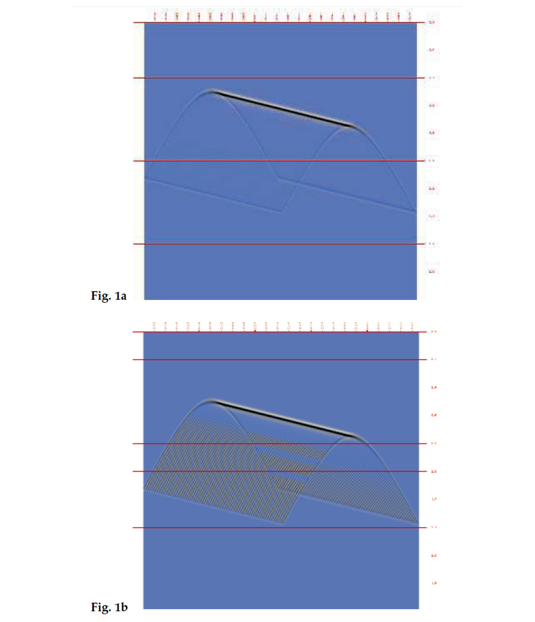
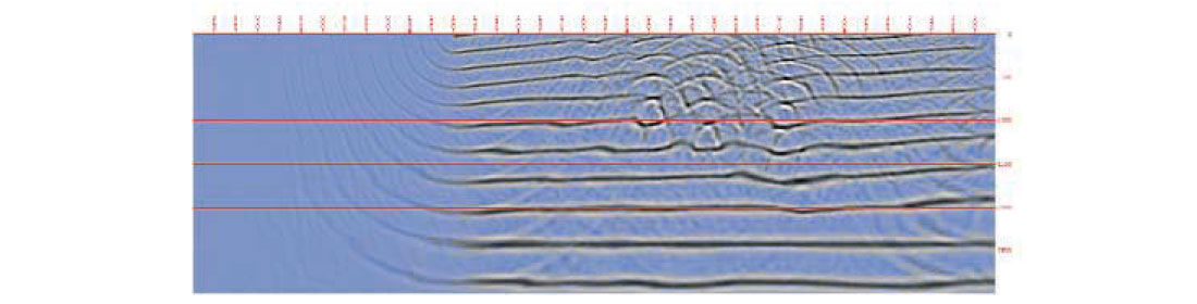
We can imagine that the shot records, plotted in the usual way, are positioned over each other in such a way that the same trace positions are above each other and the plots are shifted along the traces corresponding to the shooting time delays. Then the receiver stack is the sum of the samples positioned on top of each other. The samples will cancel out each other to a great extent, except those that lay on the envelopes of the events. These samples will be in nearly the same phase and in the summation process will have an amplified effect. Fig. 1a shows a synthetic receiver stack. The trace spacing is 25m and the wavelet is a 50 Hz Ricker wavelet. It has been created from a single hyperbola, by continuously shifting the hyperbola sideways and down and adding the shifted result to the stack. The hyperbola has been shifted 1 trace at a time, i.e. the stack corresponds to a case where every station has been shot. Assuming that every second station has been shot, i.e. the hyperbola is shifted 2 traces at a time, the receiver stack will look like the one on Fig. 1b. The heavy line is the envelope, representing the image of a flat reflector under a plane wave illumination. In order to get a less noisy stack, the shots must have a high spatial density or they should be interpolated.
Since in the stacking process most of the energy cancels out, the stack represents only a fraction of the geology. In fact, it represents a “one sided view” of the geology. The synthesized receiver stacks are usually noisier than CDP stacks, because they create the image not so much by adding what is wanted, as it happens with CDP stacks, but by canceling out what is not wanted; and most of the energy is not wanted for a single illumination. On the other hand, now we can look at the geology from different directions, and this may be very useful, regardless how noisy the picture is. In fact, small geological discontinuities may show up as mild curvatures on a CDP stack, while the same discontinuities may be very distinctly visible under a properly tilted illumination.
The controlled illumination has a close relation with common offset stacks. Imagine the following simple, ideal situation. A horizontal reflector, buried under a constant velocity overburden, is illuminated with a tilted plane wave. In that case the image will be created by ray passes which have a constant offset between their point of penetration into and their point of emergence from the earth. This fact shows that the images resulting from plane wave illuminations with different angles could be used in AVO investigations.
Problems related to the receiver stack.
Unwanted energies at the two extreme records don’t cancel out completely in the stack, and similarly, the cable ends show up in the stack as non-existent seismic features. These problems can be practically eliminated by tapering off the cable ends and entire shot records at the ends of the line.
If the shots are not fired at each trace position then the cancellation of the energy is not complete and the envelope is not smooth. If the shots are fired at every second station then the stack is still near perfect. If the shots are fired at every fourth station, then the noise becomes substantial.
The problems related to the short cable length are more evident in half spread arrangements. In fortunate cases, like in marine surveys, the half spreads can be easily extended into full spreads by using the shot-receiver reciprocity principle. We used this trick in the case of the Marmousi model.
Generating the Depth Section
(The holographic method)
CDP stacks represent a zero-offset image of the geology. These stacks can be considered as the boundary values, recorded on the surface, of the wave field generated by exploding reflectors. Hence the geological image can be computed by solving the wave equation with these boundary values. This is post-stack migration.
In the case of a receiver stack the same is not true: the depth section is not the backward propagated receiver stack. In fact, since the receiver stack was generated according to a shooting time schedule, the depth section cannot be calculated without using simultaneously both the stack and the firing schedule.
The depth section in that case will be generated by the correlation of two wave fields as follows.
We propagate the shot wave, generated according to the firing schedule, from the surface into the ground. We call this wave the reference wave. We also propagate the receiver stack, but backwards in time. We will call this wave field the seismic wave. This means that we generate the reflected waves, but given the nature of the data, we have to do that backwards in time. In this way we will have both the downward projected shot wave and the upward reflected wave at all times and at all positions.
For any given time t, let us superpose the “snap shots” of the two wave fields as recorded at time t. Wherever the two way fields coincide, there is a point of a reflector, which at that time t reflected the reference wave and created the seismic wave. Hence, correlating the two wave fields we will detect points of reflectors. A point of the reflector in this correlation process will be represented by its position in space and the intensity of the reflection, which, by definition, is some value related to the correlation.
The correlation process can be done in the frequency domain. In our computer program, used to process the Marmousi model, the correlation was done in space on the snapshots of the wave fields.
The described “decoding” method, for evident reasons, is also called the holographic method. This particular implementation of the method, where the shot wave is computed from the wave equation, will be called the shot wave method, to distinguish it from the eikonal method that is using arrival times instead of the reference wave. We will not discuss this latter possibility.
The maximum wave number in the decoded depth section will be twice the maximum wave number in the reference and in the seismic waves. (Assuming that the inputs to generate the two waves have the same frequency maximum that would be normally the case.) If the migrations use the theoretically coarsest possible grid, then the depth section has to be created on a twice as fine grid. This interesting situation is analogous to the Doppler effect: if we imagine that we are travelling with the reference wave, we see the incoming (time-reversed) seismic wave having its frequencies doubled.
We did not see this interesting fact, i.e. the need for a finer grid, being mentioned in the literature. The reason evidently is that usual numerical schemes, in the case of non-constant rock velocity, use a substantially finer grid to start with than the theoretically coarsest possible Nyquist sampling rate in space. We use a proprietary numerical scheme to solve the wave equation. This scheme can use the theoretically coarsest possible sampling rate in both space and time and has no directional sensitivity. This is achieved by performing the calculations in the 6-dimensional (x, y, z, kx, ky, kz) space, where the problems related to discontinuities in velocity on one hand, and movement of wave undisturbed by grid orientation on the other hand, have been decoupled. Under such conditions, the paradoxical need for a finer grid, to generate the actual depth section on a twice as fine grid, immediately becomes evident.
At different times different points of the reflectors may be revealed. The entire depth section will be the superposition of all detected reflector points. In mathematical terms, the depth section will be the sum of all correlations at each point.
Note that with a single illumination not the entire geology will be revealed in this way because some reflectors may not even have been illuminated. Also, the intensity of the reflectors will depend on the intensity of the illumination and the illumination angle. This will be clearly visible on the examples.
Sample Impulse Responses
In order to get a deeper insight into the imaging methods, it is usual to study the impulse responses of the methods. These impulse responses usually mean the images created by a single spike on the input data, assuming constant velocity. As we will see in our particular case, using a single spike may be not the best method for investigating these kinds of special effects.
In the case of controlled illumination not only the input spike is required but the illuminating wave front (or shooting schedule), as well.
In the first example we assume that the illuminating wave front is a horizontal plane wave and the receiver stack is a sequence of periodical spikes at the same location. The depth section is shown in Fig. 2a: it is a set of upright parabolae. In effect, the parabola has the distinguishing property that it reflects a plane wave into a single point, called the focus. Note that the parabolae reach the horizontal elevation at 45° angles.
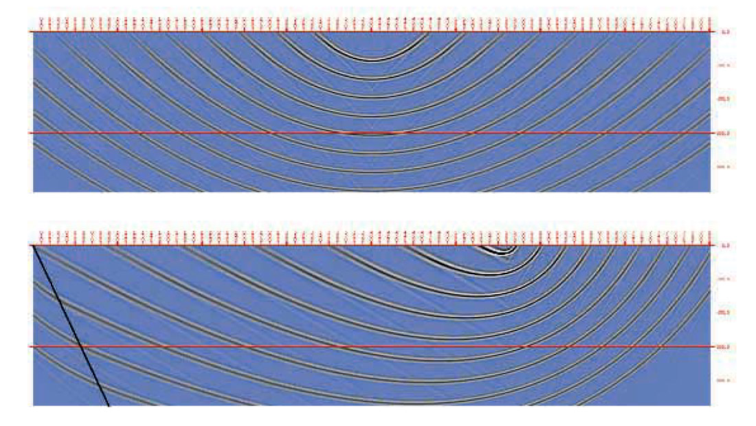
Evidently, there are some problems and artifacts on the image, but, strangely, the problem is not in the principles of Controlled Illumination or in the mathematical algorithm. The problem is in the model itself. It is true that a parabolic reflector will project a beam, arriving parallel to the axis of the parabola, into its focal point. And this focused energy, if the focus happens to be located at one of the receivers, will be recorded as a spike at this point. But that is not all the energy that will be recorded in the process: the other geophones will also record some energy projected along the surface (we are not talking about ground roll). Those recordings will be straight lines directed towards the spikes. If we only use the spikes in the process, the image will be not complete. In fact, most of the damage is done to the parabolae close to the surface.
The image can be viewed (in fact, it is) as the intersection, created in time, of a downward moving plane wave and an expanding circle. The points of the parabola, closer and closer to the elevation, are intersections of horizontal planes with circular arcs closer and closer to the vertical direction. Strange as it may appear, the computation of a reflector dipping at 45° involves a wave front dipping at 90°. Therefore, it is evident that the computation of this depth section required a numerical scheme not limited by the dips of the propagated wave fronts. In fact, the proprietary wave equation solver of Adler Mathematical has the same negligible error in all directions. In constant velocity media its dispersion error is about 5cm/km in the seismic frequency range.
In the second example we assume that the receiver stack is again the same periodical sequence of spikes - but this time the illuminating front is a plane wave with a 30° tilt. The depth section itself will be a set of parabolae again with the same 30° tilt as the illumination. The depth section is represented in Fig. 2b. Note again that the spikes do not represent a complete physical experiment and the depth section is accordingly distorted. The black line on the left shows the limits of the shadow area not swept by the incoming plane wave. The events on the left, in the shadow zone, are useless noise.
Consolidating the Various Projections
If several depth sections have been created with different illuminations then a composite depth section can be created by “superposing” the individual sections. There may be a number of ways to do the superposition. The simplest way is simply adding the migrated sections sample-by-sample, i.e. samples in the same space locations are summed.
Of course, if wrong velocities are used in the imaging process, the various images may not fit together perfectly, even if the numerical method honours all velocity variations. This may provide guidance for the processor to correct the velocity.
Limitations of the Controlled Illumination
In this section we will shortly summarize some problems. They will be visible in greater detail in the Marmousi Model figures.
Multiple illumination
In all our discussions we have tacitly assumed that each point in space is illuminated only once by the incident wave front, i.e. each point reflects energy only once. This is not true in general and it is possible that some points are multiply illuminated. (We are not talking about the usual multiple problems generated by unwanted echoes.) This may occur even if the shots generated a nice and smooth wave front on the surface. There are two reasons why this may occur:
- inhomogeneities of the velocity field may cause diffractions, which act as secondary wave front
- shock waves created in a low velocity region by a front propagating in a higher velocity region act as secondary wave front; the opposite situation is equally possible: the wave front travelling in a low velocity region can have unwanted effects in high velocity regions.
These multiple illuminations will create non-existing events, i.e. noise on the depth section. To explain the effects in more detail, let us consider the simplest case of two simultaneous shots. The first shot fired at point P1 will create a reference wave field what we denote by R1. The reflection will create the seismic wave field S1. The depth section will be obtained by the correlation of these wave fields and symbolically we will denote the result as a “star product”:
D1 = R1 * S1.
D1, by definition, as the result of the correlation, is the depth section recovered from the shot at point P1. Similarly, a shot fired at an other point P2, will lead to the depth image
D2 = R2 * S2.
The depth section created by the superposition of the two images will be denoted, again symbolically only, as
D = D1 + D2.
The question arises whether it is possible to combine the two shots into a single shot, with a reference wave denoted by
R = R1 + R2
in order to obtain the combined depth section D. i.e. we would like to correlate R1 + R2 with S1 + S2. Since the correlation process is linear and associative, we can symbolically describe the process as
| (R1 + R2) * (S1 + S2) | = | R1 * S1 + R2 * S2 + R1 * S2 + R2 * S1 |
| = | D1 + D2 + (R1 * S2 + R2 * S1) | |
| = | D1 + D2 + noise. |
Note that the first two terms in the result, D1 and D2 give exactly the desired combined depth section, but the other two terms represent noise: they are events created by correlating the wrong seismic wave with the wrong reference wave.
The multiple illumination cannot be avoided in general situations. Its effect will be diminished by superposing depth sections resulting from different illuminations: the noise will show up in different positions and therefore will be not enhanced in the superposition process.
Non-uniform illumination
The intensity of the events on the created depth section will depend not only on the incidence angle of the illuminating wave but on the energy of this wave at this point, which in turn depends on the focusing effects of the medium through which the wave traveled. There may be points or slopes that cannot be seen at all.
Advantages of the Controlled Controlled Illumination
CDP stacking can do major damage to the data by necessarily using average stacking velocities. Also, as we know, the traces in a CDP record may come from different points of the reflector, i.e. a so-called CDP record is not always a truly “common” depth point record. This will smear out the eventual discontinuity of the reflector. Since the controlled illumination is using a physically correct, velocity independent stack for imaging, the process has a great robustness and preserves the discontinuity of the reflectors. By this we mean that even if in the imaging process inaccurate velocities are used, the major structural features of the section will be retained.
Let us shortly summarize here the major advantages of the controlled illumination:
- the input to the migration is physically correct, and does not have the smearing effects of other stacking methods;
- using focusing, it is possible to enhance the sharpness of the image in a desired area;
- he created image is very sensitive to directional effects; in this respect it has the advantages of common offset stacks;
- using proper illumination angle, it is possible to “filter out” or “highlight” events.
The Marmousi Model
The Marmousi Model consists of a velocity model and a corresponding synthetic (computer generated) seismic survey produced by the Institut Français du Pétrole. This is a public domain data set, widely used to test processing methods. The data models a marine survey in very shallow water. The modeled section is 9200m long and 3000m deep. The model has been generated with an acoustic wave propagation algorithm. The shots range from 3000m to 8975m measured from the west side of the model. The trace offsets vary from 200m to 2575m. The shot and receiver intervals are both 25m. There are 240 shots in the survey. The model was shot from west to east. Hence a considerable part of the west side and a small piece of the east side are invisible to the survey.
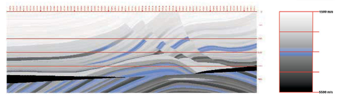
Fig. 3 represents the velocity model. The velocity varies between 1500 m/s and 5500 m/s. The model has been created to defy any CDP stacking attempt. The reservoir is the bright spot at the top of the dome like structure at about 2425m depth.
We had the experience that allowing the diffracted energy from the illuminating wave front to approach 90° increased the low frequency noise in the result, without any benefits. Therefore, we limited the maximum dip during the calculation of the illuminations, varying the limiting angle as a function of the illumination angle. This limitation does not apply to the last, focused illumination.
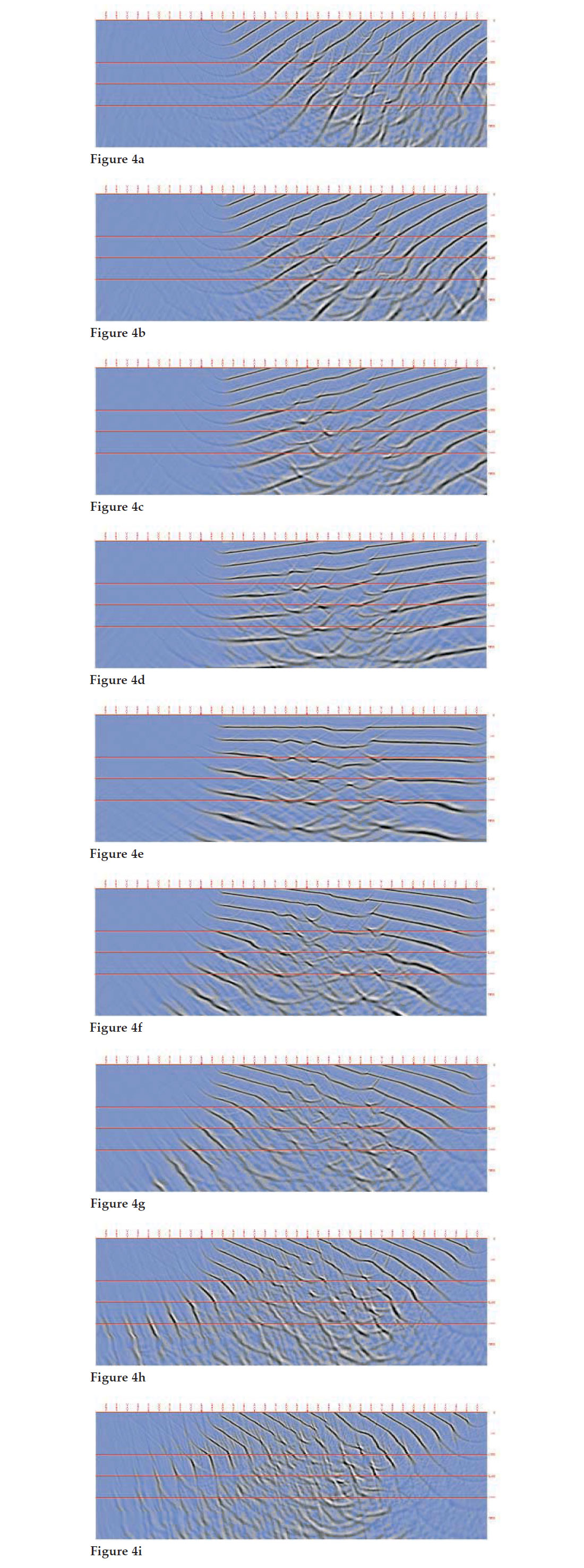
Figures 4a - 4i show superposed snapshots of the illuminating, originally flat wave fronts, projected at +28.7, +21.1, +13.9, +6.9, 0.0, -6.9, -13.9, -21.1 and -28.7 degrees. The illumination angle is defined as positive if the wave is projected from stations with lower numbers toward stations with higher numbers. The last plot in the sequence, Fig. 4j represents the wave front focused in such a way that it generates a horizontal plane wave at exactly 2425m depth. As mentioned, the calculation of this last, focused illumination has not been dip-limited. Since these plots represent depth, the wavelets are stretched on them according to the local velocity. The accuracy of the wave equation solver algorithm assured that in Fig. 4j the wave front has its maxima lined up exactly at the desired depth, notwithstanding the discontinuities of the overburden.
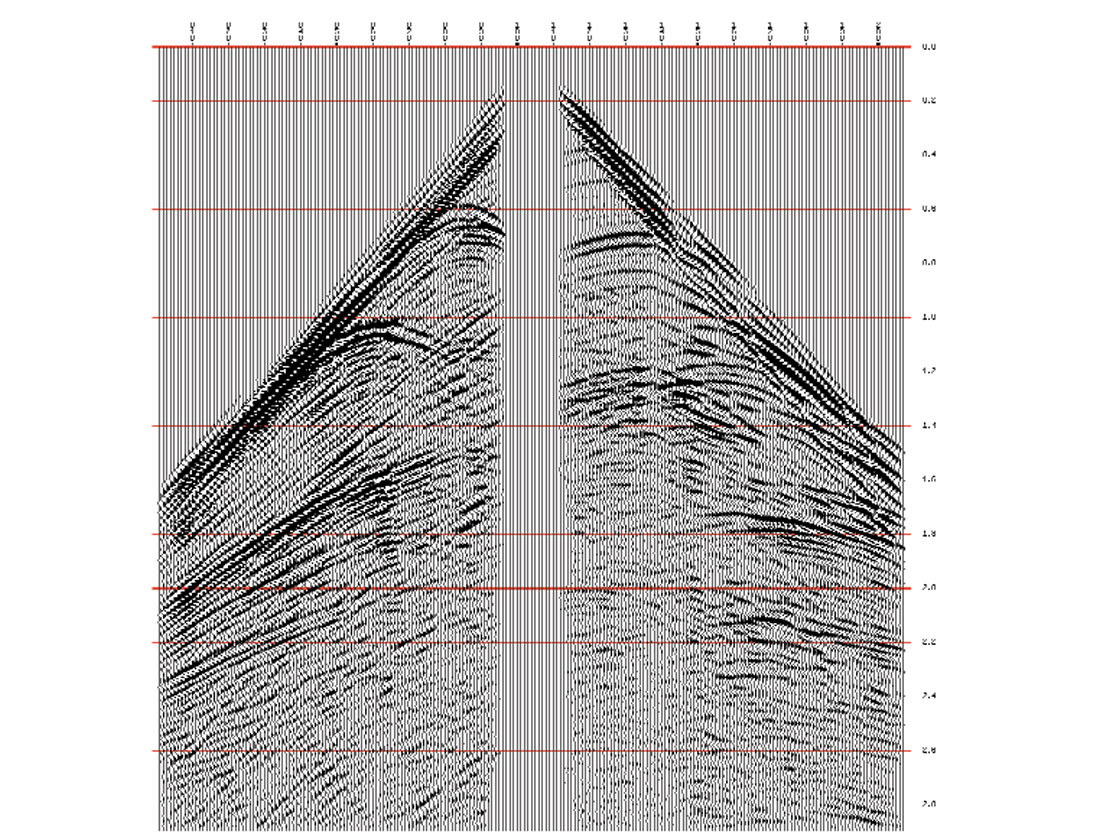
Figures 5a -5j represent the corresponding receiver stacks. Just for curiosity, Fig. 6 shows shot record no. 100. This has been extended to a full spread by using the reciprocity principle, and the cable ends have been tapered to reduce artifacts in the stack. This highlights the difficulties which could be caused by the back-scattered energy (actually all events in this record have back-scattered parts) with any conventional processing.
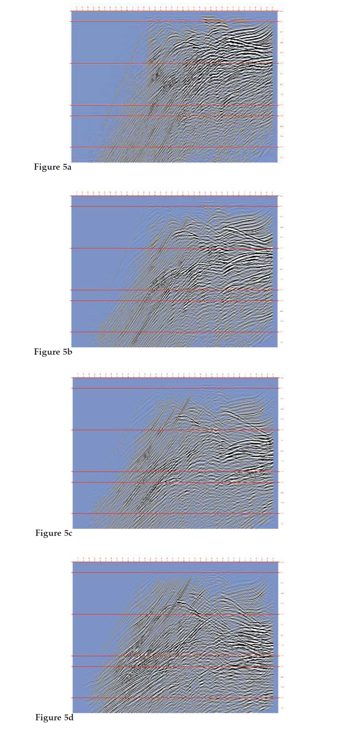
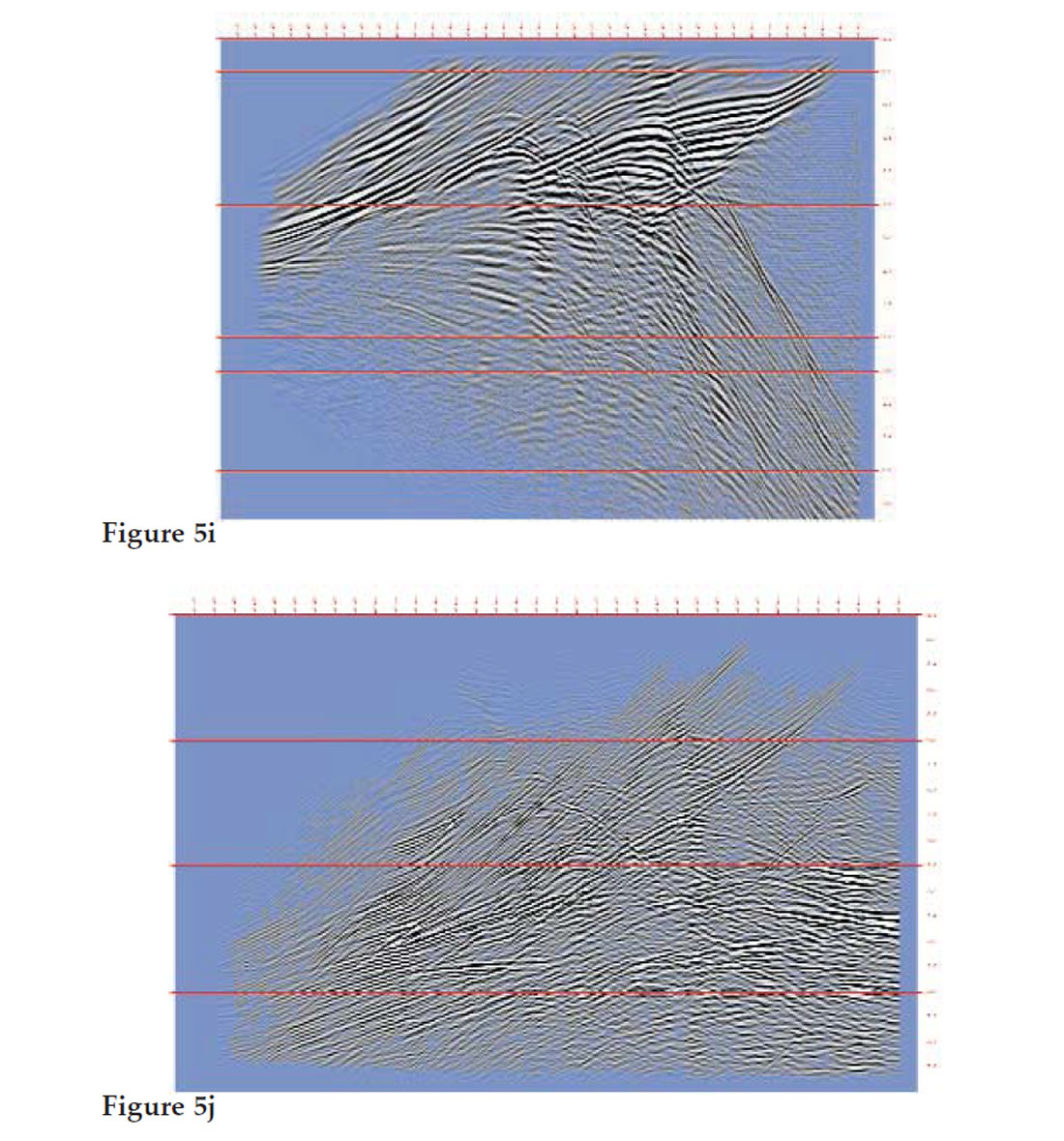
Shots with higher tilts generate longer responses and the stacks themselves become more tilted, i.e. they occupy more tilted bands in the time-offset domain, and it becomes less easy to visualize their contents. Therefore, for the purpose of display and viewing, we “shifted” the stacks back into a horizontal position. In this way they are easier to compare with each other. Note that there appears a bulk time shift on these plots.
The wavelet has a ringing character due the shallow water bottom. Most of this ringing has been removed from the stacks before migration.
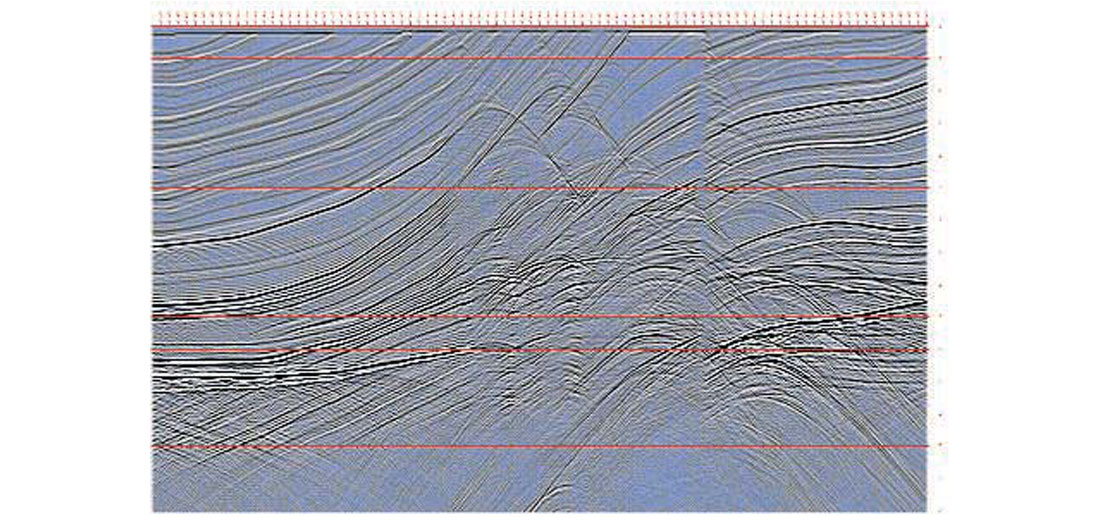
For comparison purposes, we have created a zero offset model (CDP stack) of the geology, represented in Fig. 7. The model has been generated using an 8m x 8m grid spacing. Since curved elements of the model have been poorly approximated at that scale, some reflectors are followed by a fine system of diffraction patterns. Given the accuracy of the numerical scheme and the fact that the accuracy is not limited by the dip of the wave front, these fine features show up even at later times. Since this is an “exclusively forward” model, no multiples have been generated in the process.
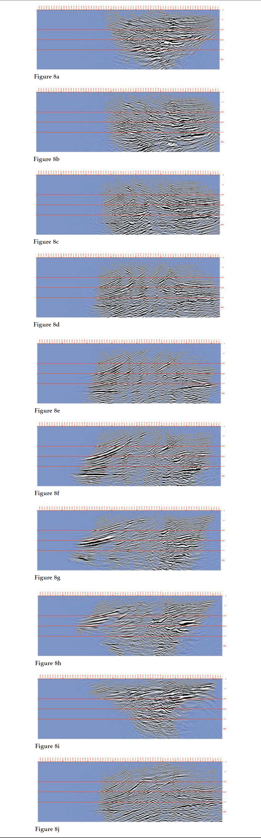
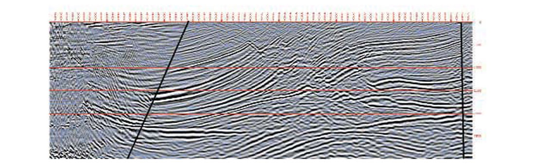
Figures 8a - 8j show the migrated depth sections without any cosmetics. Note how well detailed is the last image in Fig. 8j, created by a single focused illumination. Fig. 9 is the sum of all the previous depth sections. This section has been filtered to remove mostly the very low frequency “background” noise, created by correlating events which should not be correlated. The section also has an AGC applied to it. On this last plot, the black lines mark the boundaries of the shadow zones. The regions outside these lines are useless noise, made visible only by the AGC
Conclusion
Our conclusion, based on the results presented here, and also based on some previous processing results, is that Controlled Illumination occupies a little explored but potentially very useful area between processing and interpretation. By its nature it represents processing which can very effectively “illuminate” questionable regions during interpretation.


Join the Conversation
Interested in starting, or contributing to a conversation about an article or issue of the RECORDER? Join our CSEG LinkedIn Group.
Share This Article