Beyond Isotropy – Part II: Physical Models in LMR Space

The following is the second part of the article “Beyond Anisotropy – Part 1: A Prestack Perspective” (RECORDER, 35-7). This section provides an in depth analysis of the seismic reflection of anisotropic media, specifically using the Lambda-Mu-Rho (LMR) crossplot. In Part 1, anisotropic reflections were analyzed from the perspective of zero-offset P and S reflectivities and Thomsen’s (1986) anisotropic parameters. The concept of a zero-gradient line was defined and the different AVO classes of Rutherford and Williams (1989) were plotted on P and S reflectivity crossplot, referred to as the AVO circle.

In Part 2, the anisotropic reflection is analyzed from the perspective of a Lambda-Mu-Rho (LMR) crossplot. This allows for an intuitive feel of how reflections will change with variations in lithology, porosity or fluid fill in addition with the presence of anisotropic media. Subsequently, four distinct anisotropic AVO classes are introduced each relating to the zero-gradient line concept. Finally, the physical implications of anisotropy as it relates to fractures, is related to the LMR crossplot and basic interpretation templates are introduced.

Physical Significance

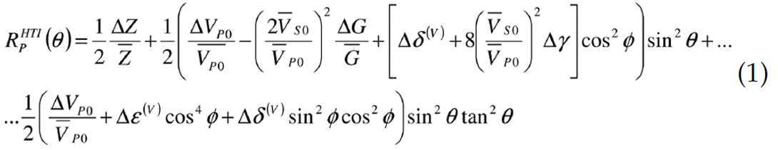
The anisotropic reflection of interest describes Horizontal Transverse Isotropy (HTI) and is given by Ruger (1997) as

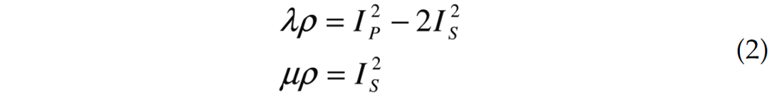
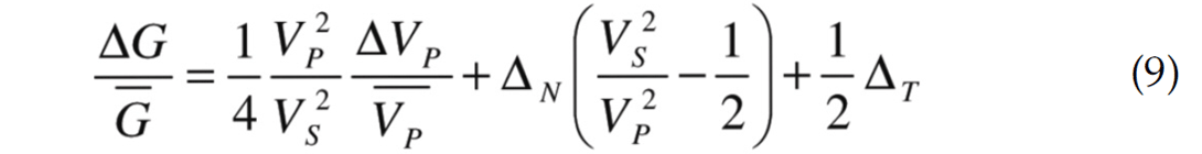
To ascribe some physical significance to the anisotropic responses described in Part 1, the reflectivity crossplot (AVO circle) is transferred to the Lambda-Mu-Rho (LMR) crossplot. The LMR crossplot is a way of comparing the incompressibility and rigidity of any rock. It can be computed using compressional and shear logs through the following equations,

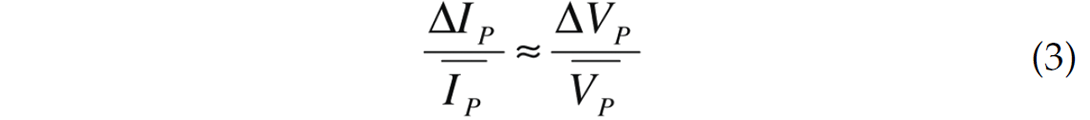
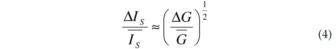
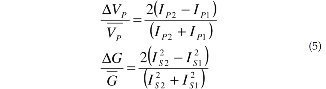
Transferring P and S reflectivity to an LMR crossplot is done by identifying lines of constant P and S impedance. With lines of constant P and S impedance, it is possible to compute lines of constant P and S reflectivity with respect to the P and S impedance of the overlying layer. The assumption of negligible density reflectivity is made so that

and

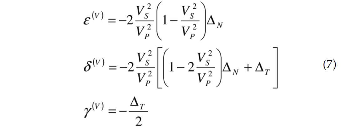
Knowing the overlying layer, IP1and IS1, it is an arithmetic exercise to compute the P and S zero-offset reflectivities through

In part one, the zero-gradient line was computed for Ruger’s VTI and HTI equation. The zero-gradient lines can be computed for both the isotropic and anisotropic cases on an LMR crossplot for a given set of anisotropic parameters.

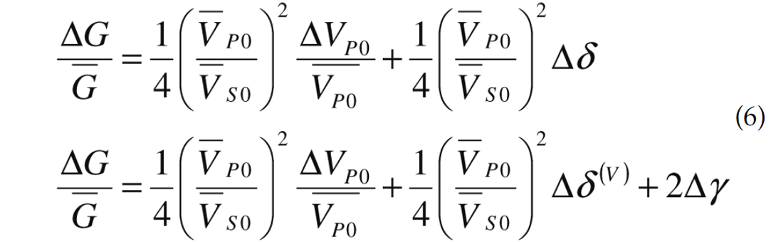
Plotting these on an LMR crossplot allows for an intuitive sense of what seismic reflections can be expected.

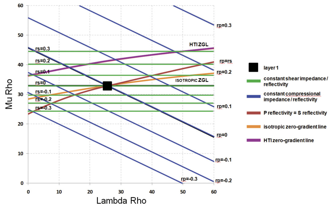
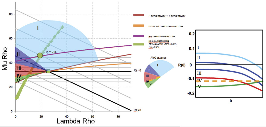
In figure 1, the blue lines are lines of constant P impedance, while the green lines are lines of constant shear impedance. The lines of constant P and S impedance also correspond to lines of constant reflectivity with respect to the overlying layer, denoted by the black square. The orange and pink curves are the zero-gradient lines for the isotropic and anisotropic (HTI) AVO, respectively. The red line has the property that P and S reflectivity are equal (Rp=Rs). With these curves the AVO reflectivity circle can be superimposed on an LMR crossplot and distinct AVO types can be identified. The position of the overlying layer (black square) defines the intersection of zero-gradient line (isotropic or anisotropic) and the Rp=Rs line. With these two lines, the five common AVO types can be identified. Type 1 is bounded by the Rp=Rs line, the boundary between Vp/Vs increases and decreases. The zero P impedance reflectivity line defines Type 2 while Type 3 is identified by zero-gradient line and decreases in P impedance, relative to the overlying layer. Type 4 AVO is the zero-gradient line. Type 5 occupies the space between the zerogradient and Rp=Rs line; a positive gradient, a decrease in Vp/Vs ratio and a decrease in P impedance.

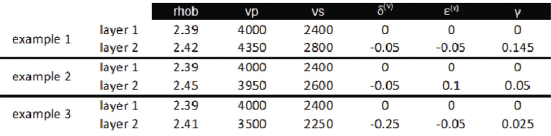
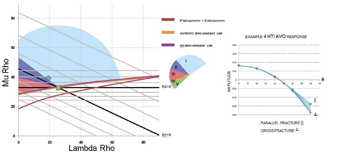
The following table shows three examples, also used in Part 1, to illustrate the effects of anisotropy on an LMR crossplot.

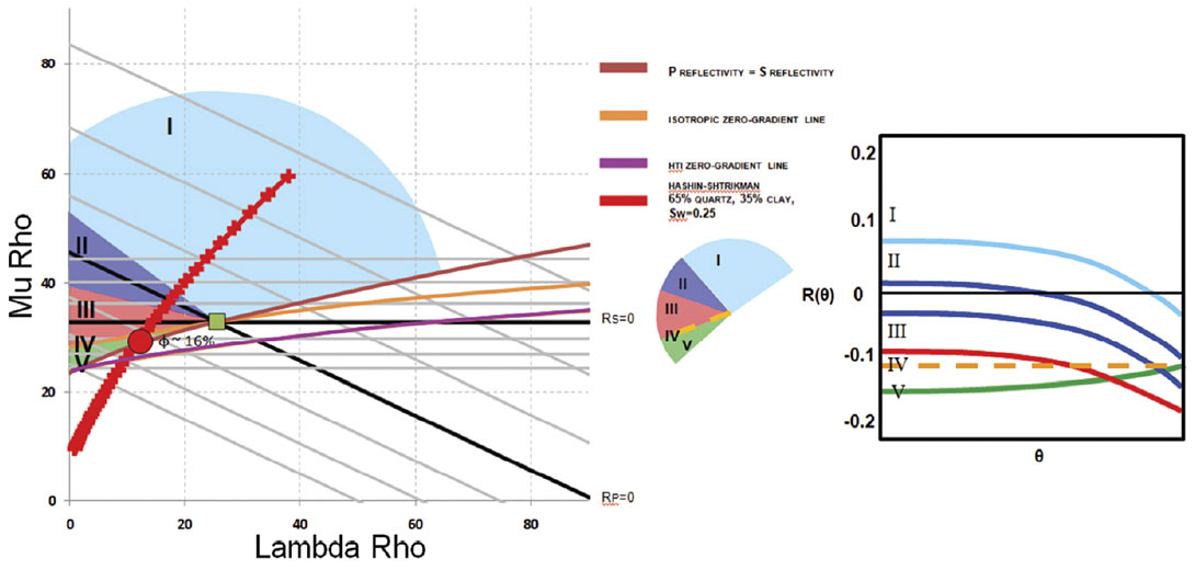
As shown by the AVO circle, the decreases in Vp/Vs ratio are the seismic signatures of interest. In figure 2, the green square represents the overlying layer while the circle is the reservoir layer of interest. In the parallel to fracture direction, the isotropic zerogradient line is used to determine the AVO type and it indicates a Type 1 AVO response with a large negative gradient. The AVO circle does not show any new information but superimposed on the LMR crossplot allows for integration of the AVO response in conjunction with rock properties providing more insight into the seismic signature. For example, in this case the green line represents a Hashin-Shtrikman (HS) rock model for a 75% quartz, 25% clay and an Sw=0.25. Layer 2 on the LMR crossplot would correspond to a 7% porosity rock of this type. Moving down the HS line towards the origin of the LMR crossplot represents increases in porosity. One can predict the amount of porosity required to produce AVO Types 2 through 5 given the same overlying layer.

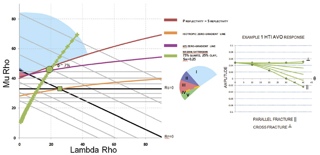
In the cross fracture direction, the HTI zero-gradient line moves to overlie the reservoir layer indicating a zero-gradient, Type 4, AVO response. The AVO circle moves to accommodate the new zero-gradient and Rp=Rs lines. The new Rp=Rs line exists to account for the new position of layer 1. The intersection of these two lines defines where properties of layer 1 would exist to produce an isotropic equivalent AVO response. In this case, as seen in figure 3, the result is a false Type 1 because although it has a negative gradient, it represents an increase in Vp/Vs ratio. Note that the HS line now indicates that much smaller porosity variation is required to produce AVO types 2 through 5.

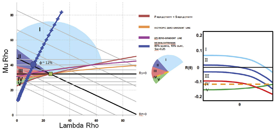
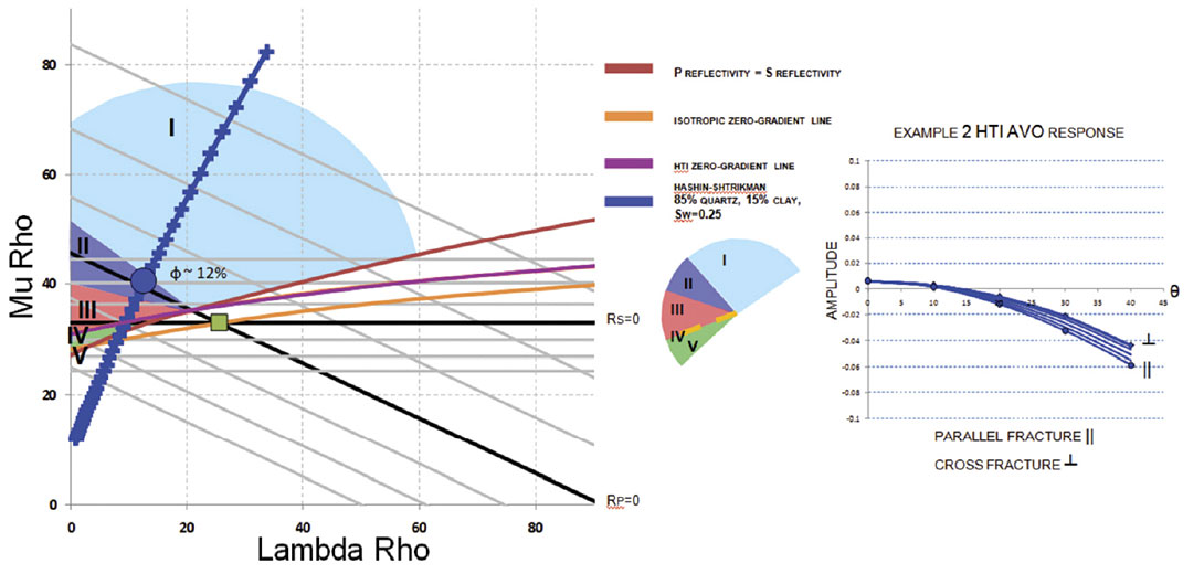
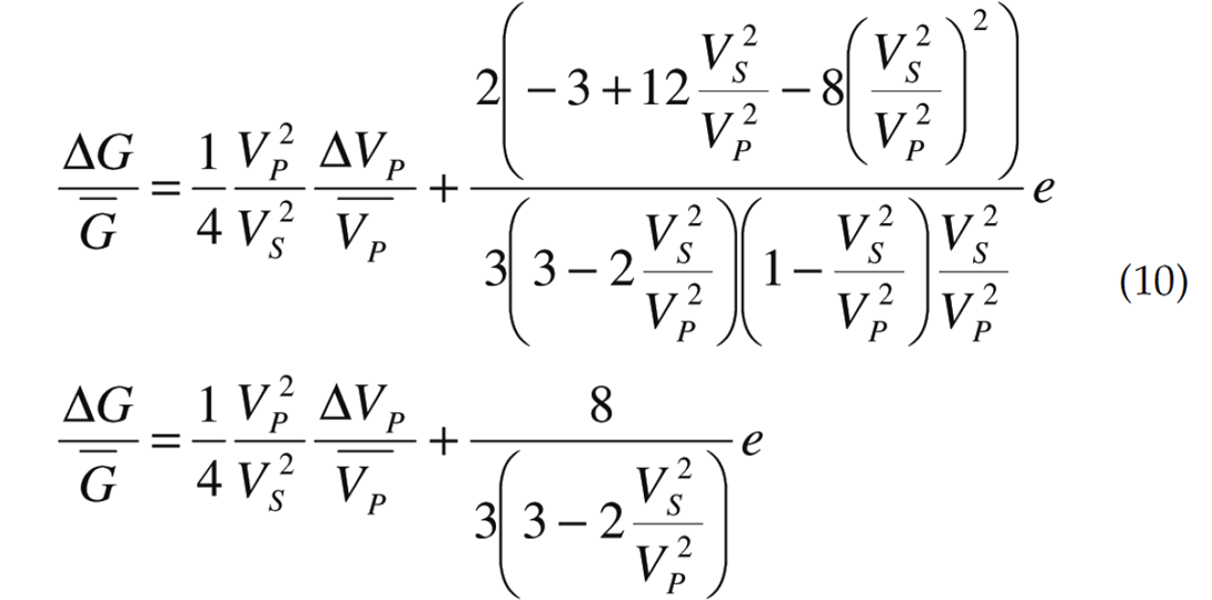
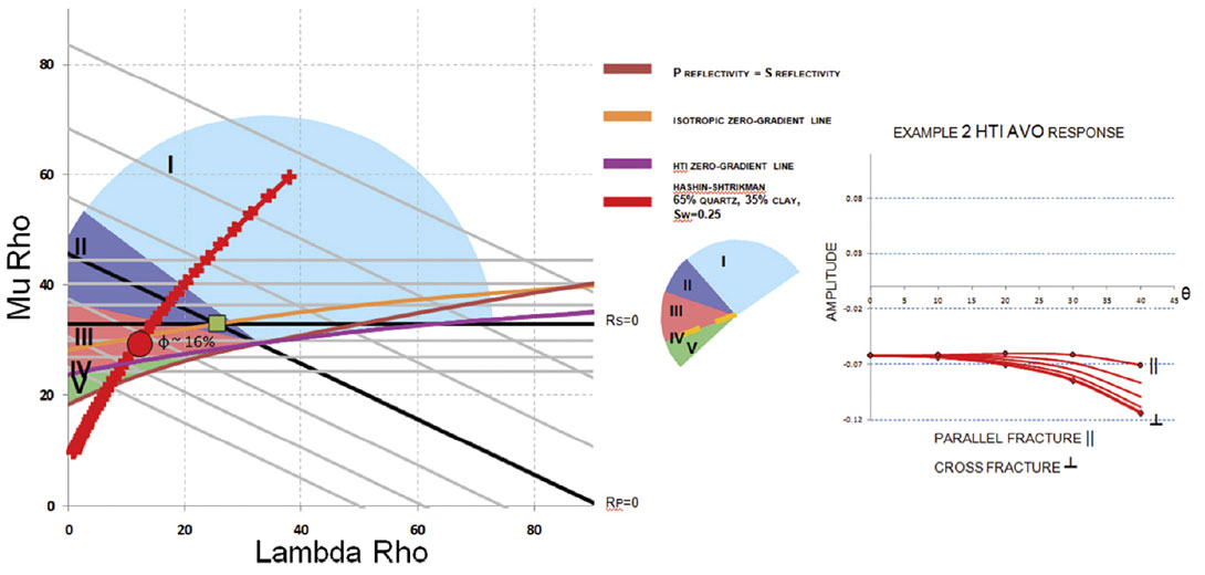
Examples 2 and 3 are seen in figure 4-5 and 6-7 respectively. Example 2 fits an 85% quartz 15% clay and an Sw=0.25 with a porosity of 12% while example 3 fits a 65% quartz 35% clay and an Sw=0.25.In addition, from Bakulin et al. (2000), the zero-gradient line expressions can be converted to accommodate the physical models of Hudson (1981) and Schoenberg and Sayers Linear Slip Theory (1995). Under the assumption of weak anisotropy, Schoenberg and Sayers normal and tangential fracture weaknesses express Ruger’s HTI anisotropic parameters as

Hudson’s model reduces to the following for gas-filled and fluid-filled cracks respectively

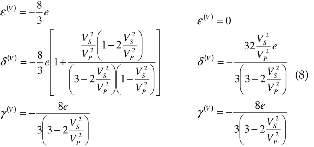
Here, e is the crack density. The zero-gradient line can then be expressed, assuming weak anisotropy and an isotropic overlying layer, in terms of normal and tangential fracture weaknesses combining equations 6b and 7:

The zero-gradient line represented by crack density, for gas-filled and fluid-filled cracks, respectively, can be expressed as

These physical models allows for a more in-depth understanding of how the change in gradient with azimuth is related to fracture weakness or crack density.

To highlight the use of the LMR crossplot consider the zerogradient line from a fracture weakness perspective where the anisotropic term is

In fact, with a standard Vp/Vs ratio of 2, the anisotropic term simplifies to

It is noticed that when Δ_T > 1/2Δ_T the anisotropic term is positive and thus the zero-gradient line will move towards positive shear reflectivities. When Δ_T < 1/2Δ_T the anisotropic term is negative and the zero-gradient line will move towards negative shear reflectivities. Thus when dealing with positive reflectivities (increases in Rp and Rs across interface) and tangential weakness is greater than half the normal weakness (positive anisotropy), one should expect a decreasing gradient when moving azimuthally towards the cross fracture direction. If the tangential weakness is less than half the normal weakness (negative anisotropy), for the same reflectivity pair the gradient should increase in the cross fracture direction. However, for a negative reflectivity pair (decreases in Rp and Rs across interface), the opposite trends will hold. With tangential weakness greater than half the normal weakness, gradient will increase in the cross fracture direction, while with tangential weakness less than half the normal weakness the gradient will decrease in the cross fracture directions.

From the perspective of Hudson’s penny shaped crack model, the zero-gradient line is defined by the crack density, e. In a gas filled crack case, with a standard Vp/Vs ratio of 2, the anisotropic term reduces to -32/45e where for the fluid filled case the anisotropic term reduces to 16/15e. In general, it is expected that the gas filled cracks will have negative anisotropy while the fluid filled cracks will have positive anisotropy. Thus depending on the reflectivity pair, the gradient may increase or decrease. However, once the reflectivity pair has been identified, the gradient polarity will be a clear indication of gas versus fluid fill, according to Hudson’s model. Note that for fluid filled cases, it is a reasonable to assume that Δ_N ~ 0 (Bakulin et al. 2000) and as such, from equation 11, the anisotropic term should always be positive. In dry cases, with Δ_N > Δ_T the expectation is of negative anisotropic terms. This agrees with Hudson’s model.

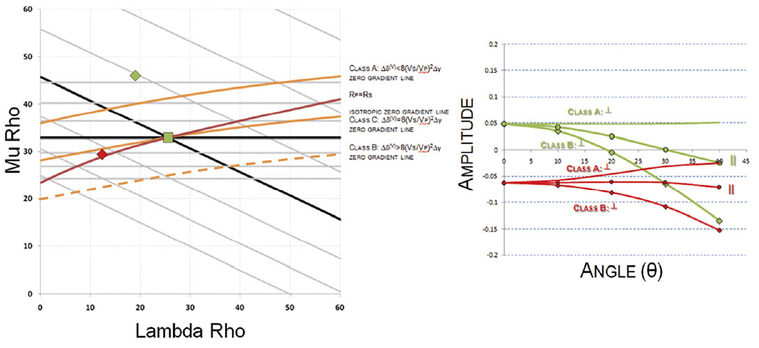
In general, as summarized in figure 8, if the isotropic gradient term is accounted for, the residual anisotropic gradient will be of:

Class A: positive when magnitude of Δδ^(V) < 8(Vs/Vp)²Δγ

Class B: negative when magnitude of Δδ^(V) > 8(Vs/Vp)²Δγ

Class C: zero when magnitude of Δδ^(V) = 8(Vs/Vp)²Δγ

As pointed out by Goodway et al (2010), there is gradient ambiguity in Ruger’s HTI equation. Because δ^(V) and γ are of opposite signs, there exist combinations where the anisotropic terms will be zero, i.e. Class C when Δδ^(V) = 8(Vs/Vp)²Δγ . In such cases, the higher order terms neglected earlier play an important role. The higher order terms can influence the gradient in ways that are counter to what was just outlined. As such, care must be taken when assessing azimuthally varying gradients and assuming the zero-gradient line’s position on an LMR crossplot. No variation in azimuth could imply a variety of scenarios, with isotropy being just one of the possible explanations. The expected anisotropic response from forward modeling can help to resolve many potential ambiguities.

For the special case of elliptical anisotropy, there exists a crossover angle where for a given angle of incidence there will be no variation of amplitude with azimuth. This angle is given by

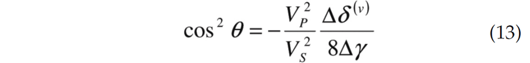
This is the angle where the higher order terms cause a change in gradient and will be referred to as Class D anisotropic reflections. Note that this will only occur when Δδ < 8(Vs/Vp)²Δγ, a consequence of equation 13; cos²(θ) must be positive and less than 1. In essence, Class D is a specific subset of a Class A anisotropic AVO response. Consider Table 2 and figure 9 which is an example of Class D anisotropic AVO. From equation 13, the crossover angle for this example is calculated to be 25 degrees. Note that the crossover angle is not the angle at which the amplitude changes from positive to negative but where the gradient is dominated by the higher order terms.

The definition of the four classes can be converted to normal and tangential weaknesses or crack density using equations 7 and 8.

Implications

In cases where isotropic inversion has been performed on a dataset and there is a seismically measurable anisotropic influence on the data, the inversion error (on account of using an isotropic instead of anisotropic inversion algorithm) can be rationalized on an LMR crossplot using the zero-gradient line.

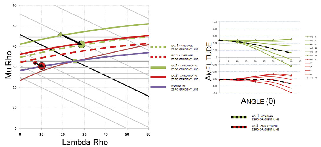
Consider example 1. The average zero-gradient line over all azimuths is assumed to lie in the middle of the isotropic and anisotropic zero-gradient lines (true for equally sampled azimuths). According to Ruger’s HTI equation, the anisotropic parameters have no influence on near offset amplitudes. These near offset amplitudes control P-impedance inversion and so the influence on any offset seismic signature can be solely attributed to changes in shear impedance reflectivity. As such, an isotropic inversion will overestimate shear reflectivity in the cross fracture direction while underestimating shear reflectivity in the parallel to fracture direction.

In figure 10, the green pyramid shows the actual zero-offset P and S impedance solution. The average AVO response would have the same zero-offset amplitude but with a smaller gradient. To accommodate the change in gradient, a new shear impedance value must be found, one that lies on a constant P impedance line. Therefore, the isotropic inversion solution will be one that is down the line of constant P-impedance towards lower shear impedance values until the appropriate amount of gradient is met. A similar argument can be followed for example 3. Since the average AVO gradient in this example is of Type 4 (no gradient), it stands to reason that the isotropic solution will be on the zerogradient line.

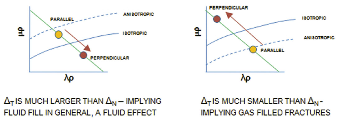
Alternatively, if azimuthally dependent inversions are performed, the changes in inversion solution may express details about fracture parameters. The differences in inversion solutions in the parallel to and cross fracture directions can represent normal and tangential weaknesses. Consider a zero-gradient line of Class A. The cross fracture direction inversion solution will move in the direction opposite to where the zero-gradient line would plot – towards larger λρ and smaller mr values. For Class B anisotropy the opposite will hold and the cross fracture solution will move towards larger μρ and smaller λρ values. From a fracture weakness perspective, Class A would imply that Δ_T is much larger than Δ_N which can be interpreted to suggest fluid filled cracks. Class B would imply Δ_N is much larger than Δ_T which can be interpreted to suggest gas filled cracks. Figure 11 illustrates the concepts for both A and B Class anisotropic reflections and their interpretations.

Note that Class C anisotropic signatures will not display any differences between the parallel and cross fracture direction inversions. Figure 12 shows Class A and B anisotropic reflections and their definitions from three different perspectives: Thomsen’s parameters, fracture weaknesses and Hudson’s crack density model. In addition, the interpreted gas and fluid effects are labeled.

Conclusion

Determining the zero-gradient lines in isotropic media allows for an understanding of AVO classes with knowledge of P and S reflectivity. The additional knowledge of anisotropic parameters also allows for predictability of azimuthally varying gradients in HTI media. Transferring this information onto LMR crossplot allows for further insight as the seismic reflection is immediately related to rock properties. Four distinct anisotropic classes for HTI media are introduced: Class A when once the isotropic gradient term is removed the residual anisotropic gradient is positive – Δδ^(V) < 8(Vs/Vp)²Δγ – Class B when the residual anisotropic gradient is negative Δδ^(V) > 8(Vs/Vp)²Δγ – Class C when Δδ^(V) = 8(Vs/Vp)²Δγ – and Class D, a subset of Class A where with elliptical anisotropy there is a gradient change. In all instances, forward modelling of anisotropic AVO response is recommended to understand the true nature of the seismic signal.