Coals and their confounding effects

Pending

Introduction

If someone were to compile a list of “usual suspects” most often blamed for processing artifacts observed on Western Canadian Sedimentary Basin (WCSB) seismic sections, high amplitude coal reflectors would be found somewhere near the top (right alongside other well-known culprits such as ground roll, anisotropy, inadequate spatial sampling and the local processing shop). To my knowledge, Coulombe and Bird (1996) were the first to publish a paper on how coals can degrade seismic image quality. They showed that some coalbeds near Simonette, Alberta acted as a transmission filter by broadening the below-coal wavelet through the interference of short period interbed multiples. After reading their excellent paper, I found myself pointing my fingers more and more often at the coals in my role as “processing troubleshooter” of problem data sets.

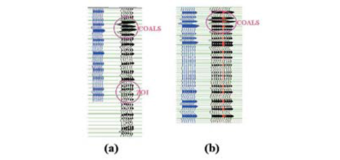
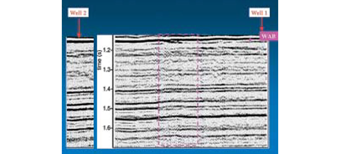
But as time wore on and my finger-pointing hands were getting increasingly sullied by coal-dust, I was becoming more-and-more bothered by the fact that I was only speculating, rather than definitively proving, that the coals were responsible for this processing artifact or the other. Fueling my unease was my observation that the presence of strong coal reflectors on the stack does not necessarily guarantee the existence of large coal-induced processing artifacts. This “good coal-bad coal” behaviour is illustrated by the two real data examples shown in Figure 1. Both data sets are characterized by very strong coal reflectors, yet the data in Figure 1b show a very poor well tie below the coals—the likely culprit almost certainly being the coals themselves as I’ll show later, while the data in Figure 1a show an acceptable (though not perfect) below-coal tie. This fact that the coals don’t always distort our sections beyond interpretability coupled with the lack of hard evidence linking the coals to observed artifacts led me to embark on a study of the how the coals can affect processing, particularly with regard to the transmission filtering phenomenon.

In this paper, I summarize my findings, some of which were reported in Perz (2000). Out of courtesy to the in-a-hurry reader, I’ll state up front what everyone really wants to know: No, I have not succeeded in removing the coal transmission filtering imprint from the data. To those of you who are still reading on, what I can offer is an enhanced understanding of how coals can influence the recorded wavefield, an approximate solution to a certain class of transmission filtering problems, and maybe an insight or two into how one might go about detecting lateral changes in the transmission filtering imprint on stacked data.

Coal-related contributions to the full elastic wavefield

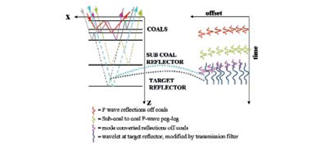
Intuition alone should tell you that coal reflectors, whose characteristic low densities (~ 1.45 g/cc) and P-wave velocities (~2500 m/s) can give rise to whopping reflection coefficients (often 0.4 or greater), can have a large influence on the recorded wavefield. Figure 2 shows the raypaths associated with what I believe to be the significant coal-induced contributions to the wavefield (a full description of all coal-related energy would lead to an impossibly messy diagram) and also the corresponding “events” as they might appear on a fictitious CMP gather. With reference to the figure, you’ll note the following events:

(a) P-wave reflection train from the coals (red wavelet)

(b) mode-converted reflections corresponding to (a) (pink)

(c) peg-leg multiple generated by a strong sub-coal reflector plus a coal horizon (green)

(d) wavelet at the target level which has been modified by short-period interbed multiples after two-way passage through the coals (blue)

Note that event (d), which illustrates the coal transmission filtering (“CTF” for short, but hopefully it won’t stick—our industry hardly needs another acronym!) effect, is the only event whose associated wavelet has penetrated through the coals down to the target level. The rest of the events may be viewed as coherent noise which may or may not overprint the zone-of-interest (ZOI) event, depending on the latter’s arrival time.

I chose to focus my study on the CTF effect largely because it seemed to be attracting a lot of attention from processors and interpreters when I started my investigation. Still, that is not to say that we can ignore the other effects listed above. In fact, I cannot even claim that CTF will be the dominant coal-related effect on any particular data set. Strong side-lobe energy produced by booming primary coal reflections (event (a)) may impede interpretation by “tuning” with the ZOI wavelet in the case where the target is located just below the coals. Depending on the strength of the side lobes, this tuning may pose more of a problem than the CTF effect. Moreover, significant peg-leg multiple energy of the type shown by event (c) is almost certainly recorded wherever there are coals, for this effect is simply an example of the classic two-bed interbed multiple problem where one of the generating beds happens to be a coal. The factors controlling the degree of success with which we can attenuate this type of multiple are well understood (e.g., amount of differential moveout on the event, amount of variation of event character with offset, etc.), and to the degree that these factors don’t permit a successful multiple attenuation on any particular data set, this type of event could easily represent the first order coal-related problem. As for the mode-converted reflection event (event (b)), Holmes and Edwards (2000) have found evidence of such energy contaminating some WCSB P-wave data sets, providing further evidence that CTF may not be the only coal-related culprit at play.

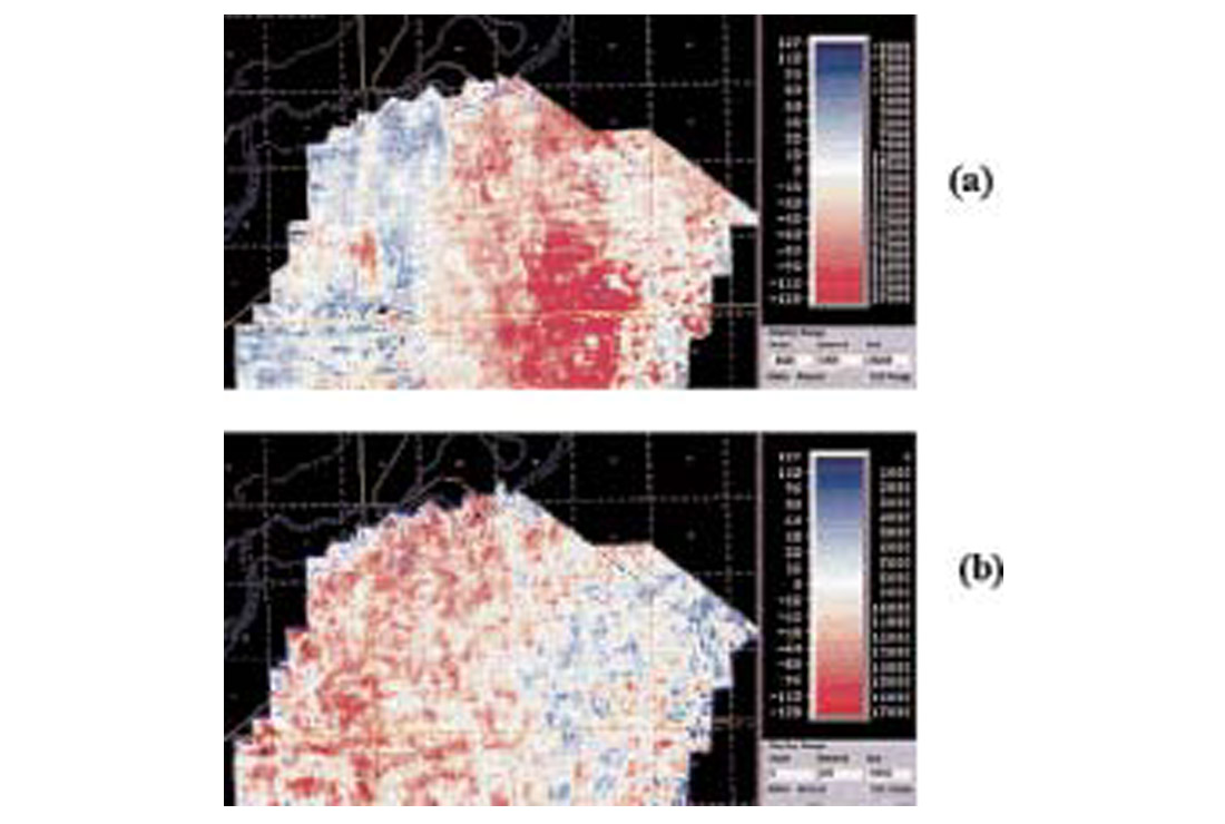
The final significant coal-related phenomenon illustrated in Figure 2 is the transmission loss introduced at the coal interfaces (see dashed lines in the raypath diagram), an effect which can significantly diminish the amplitude of the transmitted pulse. For ease of classification, you can think of transmission loss as being separate and distinct from transmission filtering, since the former is manifest as a frequency-independent pulse-scaling effect and the latter as a frequency-dependent pulse-shaping effect. In reality though, the two phenomena are inextricably entangled, as those very same short period interbed multiples which are responsible for the CTF serve to greatly compensate for transmission losses that a wavelet would sustain in a multiple-free environment (O’Doherty and Anstey, 1971). Although it’s easy to overlook the coal transmission loss effect when sections are displayed using cosmetically pleasing trace-by-trace mean scaling, we should always be aware of its presence since it can have a profound impact on the interpretation of subtle amplitude anomalies. Figures 3a and b show amplitude maps of a strong coal reflector and of a prominent below-coal horizon, respectively. The striking anticorrelation in the spatial distribution of amplitudes between the two figures clearly shows how the wavelets along the below-coal horizon have sustained differential amounts of coal-related transmission loss, depending on the reflection strength of the coals themselves.

Numerical modeling study

My investigation was guided primarily by full elastic waveform numerical modeling experiments performed using the reflectivity method, an algorithm that includes both interbed multiples and mode conversions in its response. Precise details are given in Perz (2000) but basically the approach entailed constructing an earth model that contained a detailed representation of actual coal geology based on sonic and density logs, then running the algorithm in order to capture a “standalone” below-coal wavelet at various offsets corresponding to the real survey geometry. By comparing these wavelets to those generated using an earth model that did not contain any coals, it was possible to estimate transmission filters that best shaped the “without-coal” wavelets to the “with-coal” wavelets.

Where are the mode conversions on the real data??

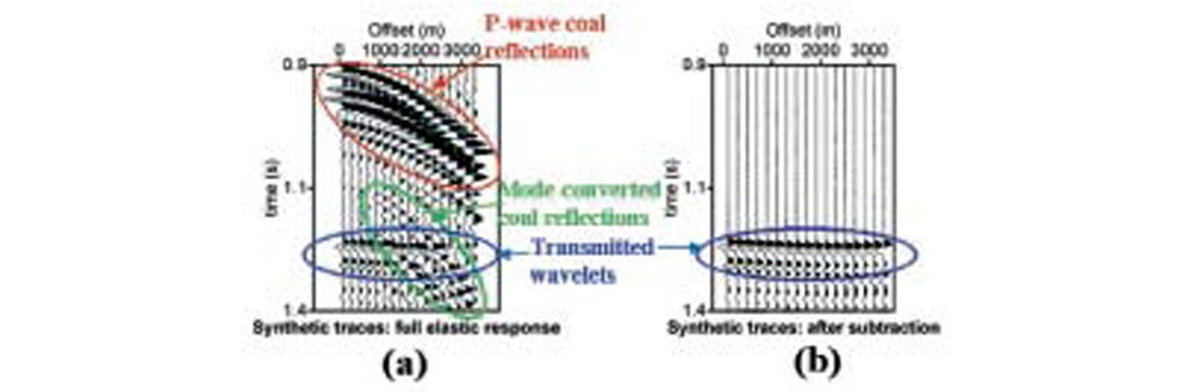
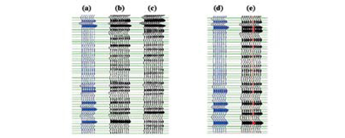
While running these numerical modeling experiments, I noticed that the synthetic seismograms were dominated by mode-converted energy which was so strong at mid-to-far offsets that it virtually swamped out the standalone captured wavelets. Figure 4a shows one of these full offset synthetic seismograms. Note how the standalone wavelets are almost completely washed out by strong coal-related mode-converted arrivals at the far offsets, in spite of the fact that I specified a compressional source and instructed the algorithm to record only the vertical component of P-wave energy (thereby ensuring that the only mode-converted energy present on the synthetics would be energy that had undergone reconversion back to P before reaching the surface). The existence of such strong mode conversions posed a problem for the isolation of the standalone wavelets; however, this was easily overcome by generating a mode-conversion “model” (in the same way that one would produce a multiple “model” as part of Radon-based multiple attenuation scheme) then subtracting it from the data (Figure 4b). What is much more troublesome about these strong mode conversions is the fact that they don’t seem to match up with what is recorded in the real world, for I did not notice much coal-related mode converted energy on any of the real data sets that I examined! Why is there such a huge discrepancy between the strength of the mode-conversions present in the synthetic seismograms versus the strength of those present on the real data sets? I do not know the answer, but one possible explanation hinges on the assumption that Q_shear is less than Q_p. Under this assumption, any energy propagating for significant distances as a shear wave would undergo severe attenuation in the real world, but not in the synthetic world which assumes an elastic earth (Qing Li, personal communication). Another possible explanation might be that the real-world wave propagation is greatly influenced by the effects of near-surface heterogeneity which can’t be accurately modeled using the reflectivity algorithm (which assumes a 1-D earth model).

Whatever the reason for the discrepancy, clearly there is some aspect of the real-world wave propagation that is not being faithfully captured in the modeling process, and at first glance this led me to question the validity of my numerical computation of far-offset coal transmission filters. However after carefully considering the two possible mechanisms which might account for the observed discrepancy (namely, near-surface heterogeneity and a greater amount of anelastic attenuation for shear waves), I don’t believe that either could greatly influence the far-offset behaviour of the transmission filters. The CTF is caused by short-period interbed multiples rattling about within the coals, and neither of these two mechanisms would appreciably affect shear wave propagation along short raypaths at the coal depth. Thus, it’s unlikely that my inability to properly model either mechanism would affect the accuracy of the numerical computations.

Numerical modeling results

I used the numerical modeling approach described above to compute offset-dependent transmission filters at six well locations around Alberta, three from the Deep Basin in west-central Alberta and three along the same seismic line in the southeastern part of the province near the town of Rosebud. Of these six wells, only one of them, so-called “Deep Basin Well 2”, was chosen at random. The rest of them were investigated based on existing knowledge that something was “wrong” with the associated 2-D seismic data sets.

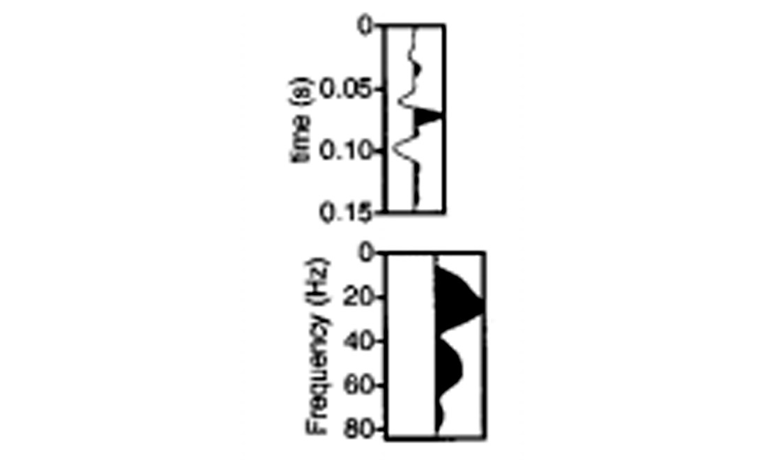
Highlights from the numerical modeling experiments are shown in Figure 5. Pay particular attention to Figures 5c and 5d. Figure 5c is a time domain display of the composite wavelet created by stacking the various offset-dependent time-domain transmission filters then performing zero-phase bandpass filtering. Figure 5d shows the corresponding amplitude spectrum. Figures 5c and 5d represent the poststack embedded wavelet that would be present in the idealized experiment in which there are no artifacts other than those associated with a zero-phase source wavelet undergoing two-way transmission through the coals at every offset. Note that this synthetic poststack wavelet embodies the composite effect of the coal operators acting on an already band-limited source pulse. Based on the displays in Figure 5 and several shown in Perz (2000), I’ll make several general comments about the character of the CTF:

• All the transmission filters’ amplitude spectra display a notching pattern at higher frequencies (Figures 5a, d).
• The primary notching frequency ranges between 40 Hz and 60 Hz depending on well location (Figures 5a, d).
• The “depth” of the notch(es) varies from mild (-8 dB) to severe (-20 dB) depending on well location (Figures 5a, d).
• The phase spectra fluctuate significantly over the signal passband (Figure 5b).
• The amount of variation of these filters with offset, though not insignificant, is small compared to the magnitude of the basic spectral notching imprint common to all offsets (compare Figure 5a to 5d, plus see Perz (2000)).
• The overall character of the transmission filters varies significantly from well to well, even over a short spatial scale—Rosebud Well 1 is only 10 km away from Rosebud Well 2 (Figure 5c).

The coal transmission filters (or “coal operators”) can be divided crudely into two types based on the location of the spectral notches within the signal passband (Figure 5d). The first type is characterized by spectral notching that occurs near the high end of the passband. In this case, the coals tend to act as a high- cut filter (Rosebud Well 3, Deep Basin Wells 1, 2). The second type is characterized by spectral notching that occurs closer to the centre of the passband. In this case, the coals tend to act as a conventional notch filter (Rosebud Well 1, Deep Basin Well 3).

Linking numerical modeling results to real data

The synthetic wavelet shown in Figure 5c doesn’t necessarily give a good measure of how CTF has affected the embedded poststack wavelet present on the real data trace that ties the well. This is because the real data will have been subject to deconvolution which may have (at least partially) succeeded in removing the coal imprint. Naturally, the question arises as to how the numerical modeling experiments might be used to measure the size of the CTF effect on real data.

Perhaps the most reliable way to ascertain that the coals are indeed causing a problem on the real data would be to extract two wavelets from the stack, one from just above the coals and the other from just below the coals, then compute the filter which best shapes the above-coal extracted wavelet to the below-coal one. The degree of similarity between this shaping filter and the numerically-computed transmission filter would provide a good indication of whether or not a coal-induced imprint was present on the real data trace at the well location. Unfortunately, it was impossible to perform a reliable below-coal wavelet extraction at any of the six well locations except for one because the wells did not penetrate to sufficient depth. As luck would have it, in the one case where I was able to extract a below-coal wavelet, the lack of strong reflectivity immediately above the coals precluded a reliable above-coal extraction!

In the absence of extracted wavelets, another way to get a rough handle on the magnitude of the CTF problem is to compute a “coal-contaminated synthetic trace” by convolving the composite wavelet shown in Figure 5c with the reflectivity series given by the well log. Since this wavelet embodies the effect of stacking various offset-dependent transmission filters, the discrepancy between this synthetic trace and the “conventional” synthetic trace obtained using the zero-phase wavelet gives you a measure of the coal-induced wavelet distortion under the “worst-case” scenario in which deconvolution has failed to remove any of the CTF imprint. If this discrepancy is similar to the discrepancy observed between the real data trace and the conventional synthetic trace, then it’s reasonable to conjecture that the coals are distorting the wavelet on the real data.

VSP information, if available, may also be used to gauge the severity of the CTF effect, and moreover, could provide a real-world validation of the computation of the synthetic transmission filters (Coulombe and Bird, 1996). Analysis of two direct arrival wavelets from a VSP experiment, one recorded just above and the other just below the coals, would give an accurate measure of the “true” coal transmission filter. Before comparing the VSP-derived transmission filter to the synthetic filter, you’d need to account for the fact that the former contains effects due to one-way propagation through the coals, whereas the latter contains effects due to two-way propagation. VSP’s were acquired at two of my study wells, Deep Basin Wells 1 and 3, but I’ve not yet analyzed the data.

(i) Deep Basin Well 1-Berland River

The Berland River 2-D data set was featured in the 1999 CSEG Multiple Workshop. Results from a VSP survey shot at Deep Basin Well l (which ties the 2-D data set) had fueled speculation that CTF may have been responsible for a certain processing artifact observed on the migrated stack. I was hoping to use the numerical modeling to definitively answer the question of whether or not the coals were the cause of the artifact. Since the well didn’t penetrate to sufficient depth to permit a reliable below-coal wavelet extraction, I had to resort to computing a coal-contaminated synthetic trace as described in the previous section. The coal-contaminated synthetic trace (Figure 6b) seems to tie the real data somewhat better than does the conventional synthetic trace (Figure 6a). Cross-correlation of the below-coal portion of the real data trace with the coal-contaminated synthetic one gives a peak value of 0.4 (Figure 6b, bottom), whereas a similar cross-correlation performed between the real data trace and the conventional synthetic trace gives a peak value of 0.25 (Figure 6a, bottom). The discrepancy between the two cross-correlations suggests that a hint of the CTF imprint remains on the migrated stack. The pressing question is whether or not it is of sufficient strength to account for the observed artifact.

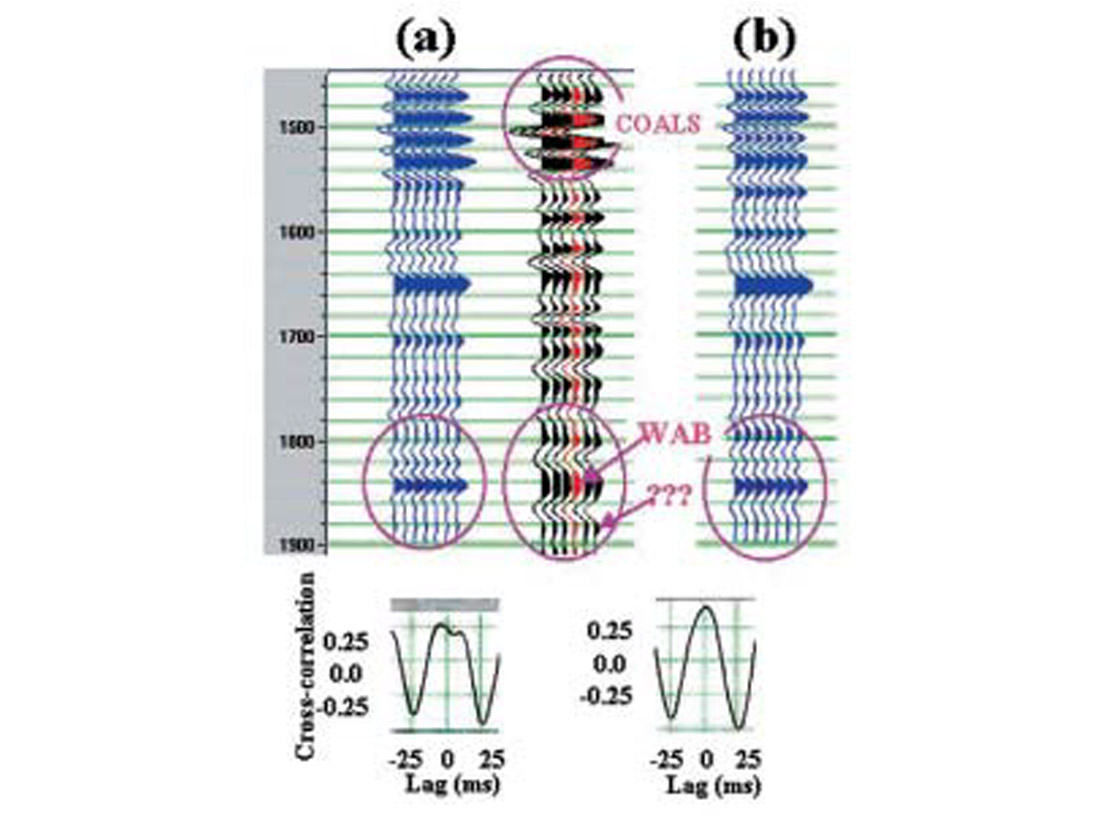
The suspected artifact is the sub-Wabamun “phantom” peak, indicated by the three question marks on the real data display in Figure 6. Note that this phantom peak, which masquerades as a base-of-porosity event, is not present on the conventional synthetic trace (Figure 6a). As for the coal-contaminated synthetic trace (Figure 6b), if you squint hard enough you might notice a very small peak at the phantom level, but the ratio of “phantom-to-Wabamun” peak strength is quite small compared to the ratio observed on the real data trace (in my opinion this ratio is quite small even on the real data, implying that the processing artifact, though undeniably present, is a weak one). Given that this coal-contaminated synthetic gives an upper bound on the possible amount of coal-induced wavelet distortion, I conclude that CTF is the not the primary cause of the artifact. However, since there is some evidence here that the coal-contaminated wavelet is (weakly) reinforcing the phantom peak, I cannot rule out the possibility that the coals are acting as a “secondary” conspirator in combination with at least one more primary culprit, for example a very fast multiple event.

In addition to imposing a very small amount of wavelet distortion, the coals are possibly causing trouble by acting as a high-cut filter. The synthetic results shown in Figure 5d for Deep Basin Well 1 suggest that the coals are performing high-cut filtering at the well location, and I observed that the below-coal seismic data are certainly lacking frequencies beyond 50 Hz. Moreover, Coulombe and Bird (1996) showed that the coals were effectively performing such high-cut filtering on their study data set which is within 80 km of Berland River. However, at the risk of appearing psychologically predisposed towards defending these coals, again I’m reluctant to assign them full blame. This is because anelastic attenuation also plays a role in attenuating these frequencies, especially when the raypath distances are large (as they are in this typical Deep Basin play), so it’s difficult to isolate finite-Q effects from CTF effects. Analysis of the VSP data might prove useful in separating out the two effects.

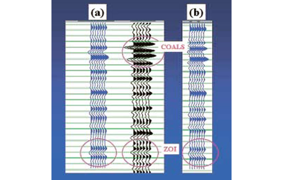
(ii) Deep Basin Well 2

The well tie at Deep Basin Well 2 was examined at the start of this article (Figure 1a), where it was presented as an example of an acceptable tie. Do the numerical modeling results confirm that CTF was indeed a relatively mild effect? At first glance that would seem to be the case, since the time domain synthetic wavelet in Figure 5c looks like a “well-behaved” zero-phase wavelet. Once again, I was unable to perform a reliable below-coal wavelet extraction, so I opted to generate a coal-contaminated synthetic trace (Figure 7b). Note that this synthetic trace is very similar in character to the synthetic trace obtained using a zero-phase wavelet (Figure 7a—in particular note the peak-trough phase relationship in the ZOI), suggesting that the CTF effect at this well location is relatively benign. However, I use the word ‘benign’ in the loosest sense, because it’s still possible that the coals were filtering out the high frequencies—again I observed that the below-coal data had a maximum frequency of about 50 Hz. Just as in the Berland River case, it’s hard to know whether the high frequency attenuation was primarily due to anelastic attenuation or to CTF.

(iii) Rosebud Wells 1,2,3

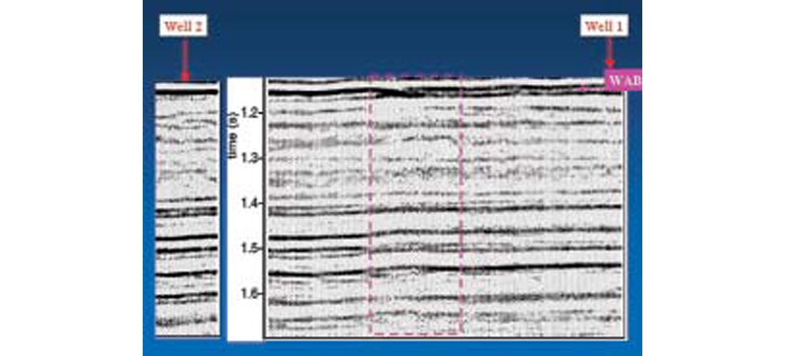
The data set which ties the three Rosebud wells seems to exhibit severe lateral wavelet instability, as evidenced by visual inspection of the stack (see Figure 8, and note that all major events seem to undergo a lateral change in character across the zone highlighted by the pink box) and also by the well ties. Of the three Rosebud wells, Rosebud Well 1 gave the worst tie with the real data. In fact, this well and its associated seismic data were presented at the beginning of this paper (Figure 1b) as an example of a particularly poor tie. Interestingly, the synthetic transmission filters computed for this well showed particularly severe spectral notching and time domain wavelet distortion (Figure 5 under “Rosebud Well 1” column). Fortunately, Rosebud Well 1 was the one well at which I was able to extract a mixed phase belowcoal wavelet from the migrated stack. Note the striking similarity between this extracted wavelet (Figure 9) and the synthetic poststack wavelet (Figures 6c, 6d under “Rosebud Well 1”), suggesting that the coals are up to no good. As discussed above, definitive proof that the coals are the cause of the mistie could only be obtained through the analysis of both the below-coal and the above-coal extracted wavelets, but as noted earlier, I was unable to perform a reliable above-coal wavelet extration. Nevertheless, I believe that the high degree of similarity between the below-coal extracted wavelet and the synthetic poststack wavelet provides strong evidence that the CTF imprint is present on the poststack embedded wavelet at the well location.

If you’re one of those geophysically unflappable types who’s not alarmed at the strong possibility that the coals are significantly distorting the wavelet at Well 1, then let me present to you the equally strong possibility that the coals aren’t distorting the wavelet too much at Wells 2 and 3. The synthetic transmission filters computed at these two well locations (Figure 5 under “Rosebud Well 2 and 3”) show less severe spectral notching, milder time domain distortion and less phase fluctuation than the filter computed at Well 1), and therefore suggest that lateral changes in coal geology could be causing the lateral changes in wavelet character observed on this data set. To summarize, the similarity between the Well 1 extracted wavelet and the computed transmission filter, the fact that the CTF is most severe at Well 1 and relatively mild elsewhere (as evidenced by numerical modeling), together with the observation that the embedded wavelet on the seismic is most distorted at Well 1 (as evidenced by well ties) all suggest that CTF is a major contributor to the lateral wavelet instability observed on this data set.

(iv) Deep Basin Well 3

“Deep Basin Well 3” was included in the study because the associated VSP data showed the existence of a strong CTF effect; moreover, a stacked section from a nearby seismic line seemed to exhibit lateral wavelet instability. The numerical modeling results (Figure 5 under “Deep Basin Well 3”), which show a high level of wavelet distortion, confirm the VSP-based observation that the CTF effect is quite severe here. The CTF seems to notch out a chunk of the spectrum located near the dominant signal frequency just like what was observed at Rosebud Well 3. Unfortunately, the nearest tie point on the real data set was over 1 km away, so I was unable to definitively link the coals to the wavelet instability observed on this data set.

Coals and deconvolution

Why has deconvolution failed to remove the severe coal imprint at Rosebud Well 1, but apparently succeeded in removing the milder imprint elsewhere along the line? To answer this question, I took the various offset-dependent synthetic transmission filters computed at Rosebud Wells 1 and 2 and submitted them to minimum phase spiking deconvolution (Figure 10). Note from the figure that deconvolution succeeds in (approximately) collapsing the ringy wavelets at all offsets on the clean synthetics at Well 1 (Figure 10a), but starts to break down in the presence of even a small amount of random noise (Figure 10b). By contrast, deconvolution produces a good result when applied to the noisy synthetic traces computed at Well 2, where the notching was less severe. The reason for the breakdown at Well 1 is best explained in the frequency domain: deconvolution is unable to estimate the depth of the spectral notches present in the raw transmission filters because these notches are getting “infilled” by the random noise.

The fact that trace-by-trace spiking deconvolution succeeded in removing the very severe coal imprinting at Well 1 in the idealized experiment where the data were noise free and the reflectivity was perfectly white raises three interesting questions about optimal deconvolution processing strategy for coal-contaminated data sets:

1. Should the input data be preconditioned using some form of random noise attenuation ? (After all, it was the presence of random noise that caused decon to break down in the synthetic tests.)
2. Would trace-by-trace decon produce better results than surface-consistent decon? (Trace-by-trace decon worked well in the synthetic tests; moreover, since lateral changes in the coal imprint don’t represent a surface-consistent effect, SC decon may not succeed in isolating them—see Perz (2000).)
3. Should the decon design window be located strictly below the coals? (The coal imprint is present on the below-coal wavelet but not on the above-coal one.)

In the case of the Rosebud data set, the answers to these questions are ‘no’, ‘no’, and ‘no’. Running prestack F-X noise attenuation, running trace-by-trace spiking decon, and/or specifying a below-coal decon design window did nothing to improve the lateral wavelet stability problem on the stack. I’m reluctant to use these Rosebud findings as a basis for making general statements about how to run decon on coal-contaminated data sets, since the three questions above really need to addressed on a data set-by-data set basis. What I will say in the way of general commentary is that I would only consider answering ‘yes’ to any of these questions if there was strong evidence supporting such an answer. Any of the three processing strategies implied by the ‘yes’ answers could introduce undesirable side effects, and these side effects could easily negate any possible benefits related to removing what could quite possibly be a very small CTF effect. Specifically, prestack noise attenuation might smear or otherwise harm the signal, abandoning surface-consistent decon in favour of trace-by-trace decon could introduce noise-related wavelet instability (which is separate and distinct from any coal-induced wavelet instability), and using a small below-coal design window might preclude the decon algorithm from collecting sufficient statistics to properly identify and remove various near-surface earth filtering effects (which could be far stronger than any CTF effects). In the end, I settled on running conventional surface-consistent decon with a large design window (encompassing both above-coal and below-coal events) for the Rosebud data set.

What about poststack deconvolution? Coulombe and Bird (1996) recommend running poststack, rather than prestack, trace-by-trace spiking deconvolution using a below-coal design window, hoping to benefit from the signal-to-noise ratio enhancement brought on by stacking. Indeed I found that this processing flow somewhat improves the lateral wavelet stability, but I also noted that running zero-phase, rather than minimum-phase, poststack deconvolution seems to give even better results (Figure 11). Compare the result in Figure 11 to the conventional stack shown in Figure 8, and you’ll probably agree that poststack zero-phase decon improves the continuity of all the belowcoal events (especially the Wabamun) across the zone shown by the pink box, and also increases the overall bandwidth. The well tie at Well 1 for this new result is shown in Figures 12a and b. For comparison purposes, I have re-displayed the poor result after conventional processing (Figure 12e) and I also show the result after poststack minimum phase trace-by-trace decon (Figure 12c). The well tie is much improved on the result after zero-phase decon, confirming that application of that algorithm has at least partially succeeded in removing the coal imprint.

On the other hand, the well tie for the result after minimum-phase decon doesn’t seem as good (Figure 12c), particularly from the viewpoint of wavelet phase. From a purist’s viewpoint, the observation here that zero-phase decon has apparently outperformed its minimum phase counterpart is rather annoying, since CTF probably really is a minimum phase effect. O’Doherty and Anstey (1971) make this claim for zero offset transmission filtering, and as for the finite-offset case, though I’ve not tried to rigorously prove the minimum phase property (any takers on this one?), the success with which minimum phase deconvolution collapsed the ringy wavelets on the synthetics in Figure 10 seems to suggest that the finite-offset coal transmission filters are (at least approximately) minimum phase. Perhaps the poststack version of the CTF effect is not minimum phase, the action of stacking various offset-dependent minimum phase filters having sufficiently altered the phase characteristics of the resulting poststack CTF imprint. Then again, perhaps the poststack CTF imprint is (close to) minimum phase, but spiking decon is getting the phase estimate wrong. In the end, it doesn’t matter why spiking decon didn’t work as well as zero-phase decon—the fact is that poststack zero phase decon has improved the result here.

In spite of these promising Rosebud results, running poststack zero-phase decon on the Berland River data set (i.e., the data associated with Deep Basin Well 1) did nothing to change the appearance of the stack other than to introduce a bit more random noise. In fact in almost every case I’ve examined where the data set is suspected to suffer from CTF-related wavelet distortion, I’ve observed that applying poststack deconvolution (either minimum-phase or zero-phase) degrades image quality. Why is the poststack deconvolution giving such inconsistent results? Certainly the signal-to-noise ratio on the stack and also the amount of good signal that exists below the coals would influence the success of the algorithm on any particular data set. But perhaps another explanation for the spotty success associated with running poststack deconvolution lies in the character of the poststack transmission filter imprints themselves. Recall that in the case of Rosebud Well 1, the CTF-related spectral notching lies well within the signal passband, while in the Berland River case it lies near the high-end of the passband (Figure 5d). It’s quite possible that in many cases where the coals impose high-end spectral notching, the composite effect of the CTF acting on an already-bandlimited wavelet serves to attenuate the signal beyond a recoverable level. This in turn suggests that poststack deconvolution probably works best in cases where the coal imprint is characterized by mid-band, rather than high-end, spectral notching.

Diagnostic tools

In spite of the fact that the Rosebud result after poststack zero-phase deconvolution shows improved lateral wavelet stability, I strongly doubt it’s perfect—careful inspection of Figure 11 shows some remnant lateral changes in wavelet character. So if we can’t always reliably remove coal-induced lateral wavelet variations, can we at least detect them? The synthetic displays in Figure 5 show that CTF can affect both the amplitude and the phase spectrum of the wavelet, suggesting that diagnostic tools tracking lateral changes in either amplitude or phase might be provide useful measurements. However, because measuring lateral changes in wavelet phase is a tricky business (it’s easy to confuse lateral changes in geology with phase changes), I prefer to examine diagnostics which exploit changes in the coal operator amplitude spectrum.

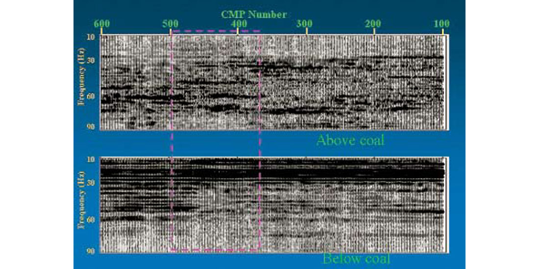
Probably the easiest and most reliable way to detect lateral changes in coal operators is by simply computing amplitude spectra for each trace then displaying them in standard stack format (Margrave, 1999), using both an above-coal and a below-coal window. If lateral changes are observed in the below-coal plot but not in the above-coal one, there’s a good chance they are due to spatial variations in CTF (observing the same lateral changes in both the above-coal and belowcoal spectra is no cause for celebration either, as this suggests that the data may be haunted by a source ghost (Hamarbitan and Margrave, 2001)). These “FX spectra” are displayed in Figure 13 for Rosebud, where it seems that they have succeeded in detecting the wavelet stability problem as evidenced by the lack of frequencies beyond 30 Hz on the below-coal plot, starting at CMP 460 and proceeding to the right.

These FX spectra, while obviously useful for detecting CTF-related spectral notching problems, suffer from two limitations. First, it’s difficult to relate any differences observed between above-coal and belowcoal plots directly to the action of the coals (rather than to Q-effects, for example) since the temporal windows associated with each of these plots typically aren’t tightly localized immediately above and below the coals. Second, detection of spatial variations in spectral notching poses visualization problems for 3-D data sets, since the F-X spectra naturally contain information at all frequencies. Thus, it would be desirable to come up with a new attribute that is better localized in time and also quantifies the severity of the spectral notching using a single frequency-independent scalar. With these considerations in mind, I’ve devised a simple detection algorithm which works as follows: First, for each sample on each poststack trace, a local amplitude spectrum is estimated by performing a short window FFT using a 300 ms window (continuous wavelet transforms may provide better localization in frequency and in time than short window FFT’s, but I suspect that such limitations in frequency-time resolution represent the second order problem, the first order one being that the reflectivity can look quite coloured over the short temporal window). Next, I compute an attribute called f_CRAP . “CRAP” stands for Cumulative Relative Amplitude Percentile (the “Relative” doesn’t really describe the attribute at all, but that capital R sure spices up the acronym!) and f_CRAP is that frequency at which the area under the local amplitude spectrum curve integrated between f=0 Hz and f= f_CRAP Hz equals 80% of the area under the local amplitude spectrum curve integrated from f=0 Hz up to some pre-specified maximum signal frequency f_MAX. In the ideal case where the local amplitude spectrum is perfectly flat, f_CRAP = 0.8* f_MAX , but in cases where the high end of the spectrum is contaminated by spectral notching, f_CRAP could be much smaller than 0.8* f_MAX . By performing such a computation for all samples on all the poststack traces, a data set of f_CRAP values is created which can be overlain atop the input stack in a display. Figure 14 shows the result for the Rosebud data set. It seems that the CRAP algorithm has succeeded in identifying the lateral changes in below-coal wavelet character (coals are at 950-1050 ms), as evidenced by the shift from higher to lower f_CRAP values proceeding from left to right across the pink box (i.e., towards the zone where the CTF becomes more severe) and also by the somewhat abrupt lowering of f_CRAP values at the coal level, proceeding from top to bottom down the display for CMP’s 450 and lower.

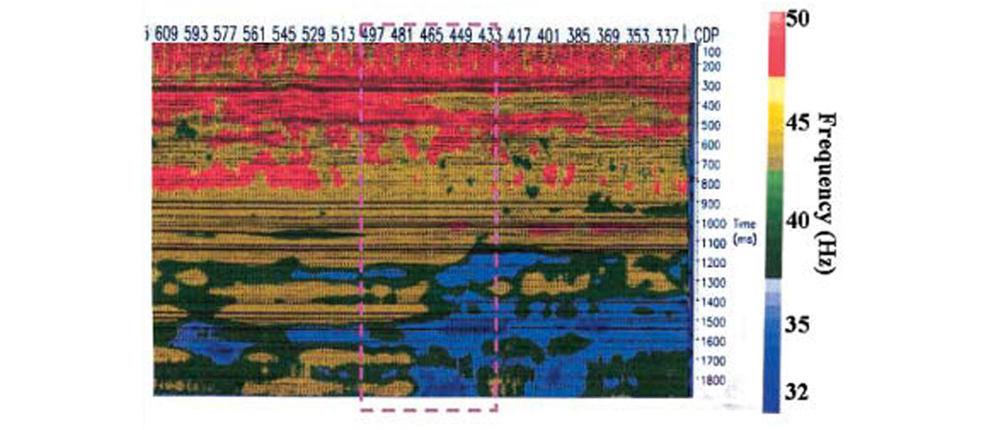
Interestingly, Figure 14 suggests that the above-coal wavelet character also changes across the pink box, which would appear to contravene my hypothesis that the coals are responsible for the lateral wavelet instability. Is this change in above-coal character real, or is it an artifact of the detection algorithm? I think it is real, since careful inspection of the FX-spectra plot (Figure 13) and also of a plot produced by tracking lateral phase along above-coal horizons (not shown here) show some evidence of above-coal lateral character change. Although I cannot rule out the possibility that there is another mechanism at play here as well as the CTF, there is so much evidence linking the coals to the wavelet instability that I would be very surprised if CTF wasn’t the primary culprit. One possibility is that the coals are indeed the sole cause of the problem, and that the above-coal character changes laterally across the region shown by the pink box because the deconvolution operators, being adversely influenced by the CTF-related spectral notching observed near Well 1, are also changing across the region indicated by the pink box.

While the CRAP algorithm has apparently succeeded in identifying the problem on the Rosebud data set, I’m still reluctant to place too much trust in its results. Since coloured reflectivity could contaminate the local spectral estimates and therefore lead to erroneous f_CRAP estimates, I suspect that the algorithm has the ability to generate “false positives”. If there is oil or gas out there waiting to be found, the last thing I want to do as a processor is to run interference by having my diagnostic tool warn the interpreter of some potentially very small (or even non-existent) coal-related problem that might not adversely affect the interpretation! And without running the CRAP algorithm through a calibration phase using several other data sets which are known to suffer from CTF-induced lateral wavelet instability, I can’t comment meaningfully on what amount of lateral change in f_CRAP values constitutes a bonafide wavelet stability problem versus what amount constitutes normal algorithmic “noise” due to coloured reflectivity. But by now you no doubt appreciate just how difficult it is to find data sets for which CTF is absolutely positively the cause of lateral wavelet instability, even if such data sets are out there in droves!

Conclusions

Several coal-related effects may significantly distort image quality of WCSB sections, namely transmission loss, transmission filtering, primary and/or mode-converted coal reflections which may overprint the ZOI event, and finally interbed multiples involving one or more coal reflectors. Synthetic experiments indicate that CTF can be a significant effect in the Deep Basin and in east-central Alberta and that the primary factor controlling the severity of this effect seems to be the location and depth of spectral notches. When the spectral notching occurs near the high end of the passband, the coals tend to act as a high-cut filter. On the other hand, when the spectral notching occurs closer to the dominant signal frequency, they tend to act more like a standard notch filter. It is difficult to definitively link the synthetic results to real-world coal-related problems without very good well control, but worst-case scenario computation of coal-contaminated synthetic traces indicate relatively mild CTF effects on two Deep Basin data sets from the viewpoint of distortion of wavelet shape. However, both of these data sets show evidence that the coals are attenuating high frequencies (though it’s difficult to isolate CTF-induced high-cut filtering from finite-Q effects). Results from the Rosebud area indicate that lateral changes in the CFT effect can result in lateral wavelet instability in the conventional stack, but that this problem may be partially overcome by running zero-phase poststack deconvolution using a below-coal design window. Poststack deconvolution has yielded poor results on several other data sets suspected of suffering from CTF-related artifacts, leading to the speculation that the algorithm works best in cases where the coals are acting as a mid-band notch filter, rather than a high-end bandpass filter. F-X spectra displays prove to be a useful indicator of CTF-related problems on the stack. A new diagnostic tool, the CRAP algorithm, shows some promise in identifying CTF-induced lateral wavelet instability but requires further validation and calibration using real data sets which are known to suffer from CTF-related problems.

Based on a limited sample space of three 2-D data sets and six wells, I would have to say that the coals have rightfully earned their place among the “usual suspects” of the processing world. However the fact that I was out “looking for trouble” at five of the six well locations means that my results can’t be used as a basis for making statistical inferences about what percentage of data sets in the WCSB as a whole might suffer from coal transmission filtering problems.

Acknowledgements

This research has benefited greatly from enlightening discussions I’ve had with various people, among them Peter Cary, Bill Goodway, Dave Hughes, Qing Li, Brian McCue, Ann O’Byrne, Mauricio Sacchi, and Xishuo Wang. I’d also like to thank Canadian Hunter Exploration Ltd., Burlington Resources Canada Energy Ltd., PanCanadian Petroleum Ltd., and one anonymous donor for the real data examples, and finally Colorado School Mines for use of their Seismic Unix plotting software.