Datums, Projections and Coordinate Systems

Accurately describing locations on Earth is essential to exploration geophysics. The interpretation of fault zones, the surface and bottom locations of a well, and the position and orientation of seismic ground control points and receivers are all dependent on being able to accurately describe where they are. Unfortunately the latitude and longitude of a location (and the height) are not enough to describe where on Earth it is. There are numerous datums and projections to which the coordinates are referenced, and using the correct one can make the difference between successful exploration and expensive legal fees. There are also numerous applications for analyzing and interpreting spatial data, all of which have different methods for representing a three-dimensional position in two-dimensional space. Assumptions are dangerous, and not all spatial data is acquired and delivered in the same way. The location of a coordinate in one datum will be different for the same coordinate in another datum. Understanding the spatial data acquisition methods and the idiosyncrasies of individual applications will allow users to take the correct action to make decisions that ensure positional integrity and accuracy in exploration geophysics. This article describes the theory behind datums, projections and coordinate systems, and highlights the importance of using the correct one for a given purpose.

Methodology

The terms datum, projection and coordinate system are often misinterpreted and misunderstood. A datum is simply a foundation and reference for spatial measurements. A system of coordinates is then used to describe those measurements relative to the datum, and a projection is the visual representation of those measurements on a different surface. There are many datums and coordinate systems, each representing a different level of accuracy in different regions around the globe. A coordinate system and its datum are therefore required to determine accurate locations, and unless a perfect scale model of the Earth is used, it will be necessary to use a projection to visually represent those locations on a different surface. The following sections describe datums and projections in more detail.

Datums

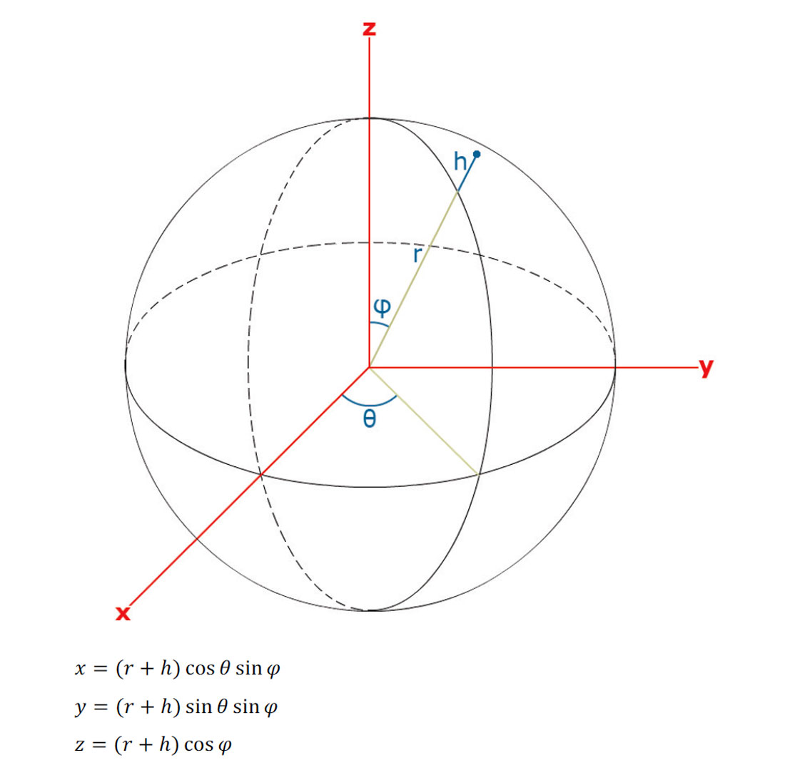
A datum is a reference frame that enables a system of coordinates to describe positions in three-dimensional space. Consider a perfect sphere as a reference frame with the sphere’s center as the origin of that frame. The sphere has a known mathematical model that can describe the position of any point at height h above its surface, as shown in Figure 1.

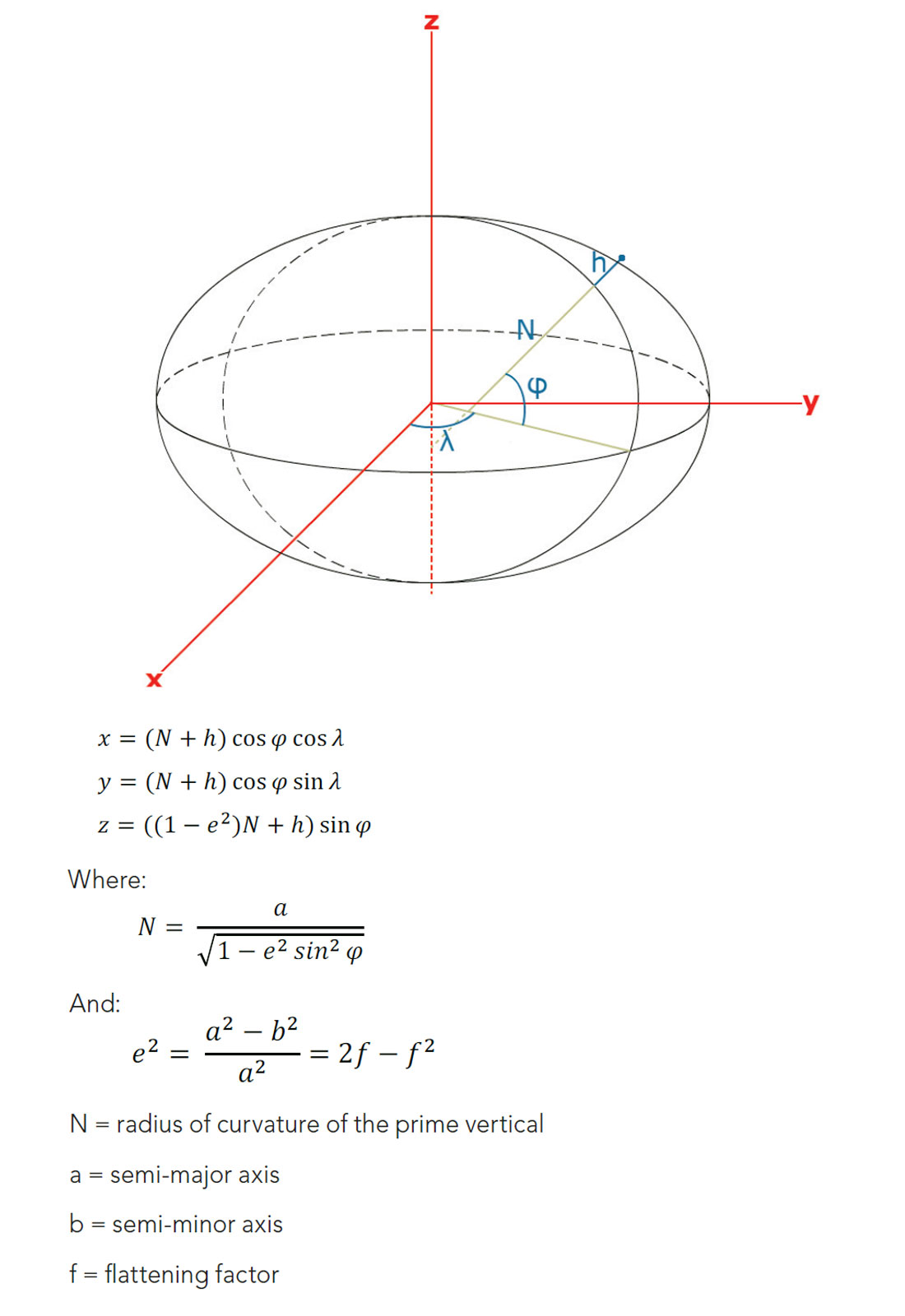
Now consider an ellipsoid as a reference frame, which also has a known mathematical model that can describe the position of any point at height h above its surface, as shown in Figure 2.

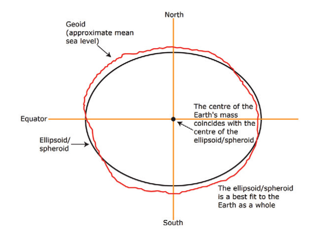
The surface and shape of the Earth is highly irregular and difficult to represent mathematically, which means ellipsoidal and spheroidal models are only approximations of the Earth’s true geometry. A more accurate representation – based on the approximate mean sea level – is called the geoid, but requires gravity measurements and the determination of the gravity potential, the theory for which will not be covered in this article.

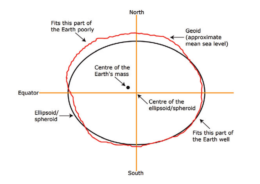
Although the ellipsoidal and spheroidal models are only approximations of the Earth’s true geometry, they can still be used to determine local coordinates with relative accuracy. For example, rather than aligning the center of the reference frame with the center of mass of the Earth, the reference frame can be shifted such that its surface coincides with the surface of the geoid in a regional area. This enables positions in the regional area to be described with greater accuracy. Figure 3 and 4 show the differences between a geocentric reference frame and a regional reference frame. While the geocentric reference frame is a good approximation of the entire geoid, the regional reference frame is usually a better approximation in a regional area (Anzlic Committee on Surveying and Mapping (ICSM), 2016).

Two horizontal datums are often used in Canada today. They are the North American Datum of 1927 (NAD27) and the North American Datum of 1983 (NAD83). NAD27 is a regional datum based on a reference ellipsoid that was determined in 1866 (Clarke 1866). NAD83 is a geocentric datum based on a reference ellipsoid that was determined in 1980 (Geodetic Reference System 1980), over one hundred years later (Statistics Canada, 2015). Although NAD83 is a geocentric datum, its reference ellipsoid is a more accurate representation of the Earth’s geometry in North America because it was determined using a combination of terrestrial and satellite Doppler measurements. NAD83 is the official datum of the International Union of Geodesy and Geophysics (IUGG) and is also the basis for the World Geodetic System of 1984 (WGS84), which is used by the Global Positioning System (GPS). Thanks to improved satellite gravity measurements, the differences in height between the geoid and the reference ellipsoid (geoidal undulation) can be used to provide a more accurate vertical datum, which is important for determining three-dimensional positions (e.g. latitude, longitude, height) (Hofmann-Wellenhof & Moritz, 2006).

Consider a planned well whose surface location has a coordinate of latitude 58°0'0.000 N" and longitude -133°0'0.000 E". The geodesic distance between the same coordinate in NAD27 and NAD83 at this location is approximately 113 m. Even if the coordinate of this well is correct, using the wrong datum could have significant financial, legal, regulatory, and/or environmental implications. For example, the planned surface location of the well could appear to be outside its mineral surface lease (well pad) in an area not authorized for surface activity, potentially requiring a redesign of the well pad resulting in further land contract negotiations and/or environmental assessments. Making a similar error during or after drilling could result in failure to reach an intended mineral target, or produce from a zone outside a mineral lease, possibly resulting in a dry well or mineral trespass, respectively. The consequences of mineral trespass vary, but the Alberta Energy Regulator introduced a penalty of $50,000 per occurrence. In addition to the penalty, compensation may be owed to the Crown for the value of any minerals obtained during trespass (Alberta Energy Regulator, 2016).

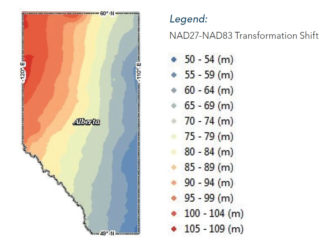
Figure 5 is a contour plot showing the approximate transformation shift in meters between a coordinate in NAD27 and the same coordinate in NAD83 across the province of Alberta. The magnitude of the transformation shift increases in the North-West direction, continuing into British Columbia, Yukon, and Alaska.

Projections

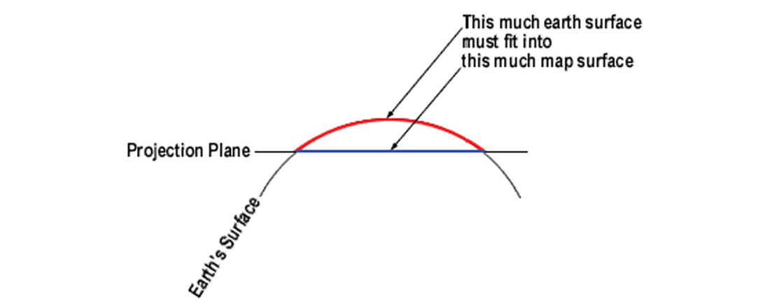
A projection is a two-dimensional representation of a three-dimensional surface. Paper maps, web maps and mapping applications represent the Earth in two dimensions and therefore require spatial features on its surface to be projected. However, projecting these spatial features will always induce distortion either by area, shape, scale or angle. A perfect three-dimensional scale model of the Earth is the only way to eliminate all four distortion types. Figure 6 shows one example of how distances on the Earth’s surface will be shortened after projecting it onto a two-dimensional plane.

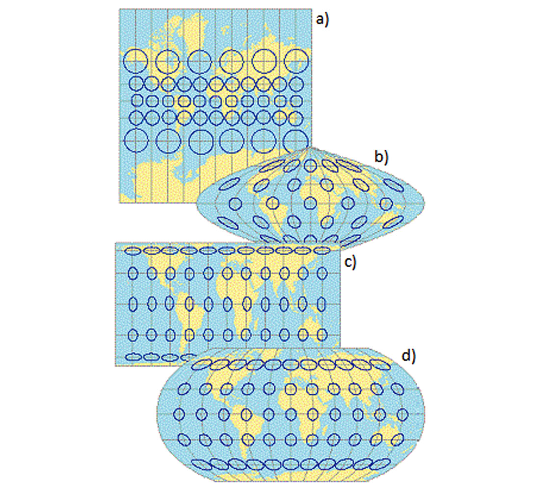
There are many different projections available, and using an appropriate projection depends entirely on the purpose and function of the map. Some projections maintain accurate geographic areas, while others maintain accurate shapes and angles, such as the Transverse Mercator used for nautical navigation. Tissot’s indicatrix is a method used to illustrate these projection distortions, whereby uniform circles are placed at fixed positions on the surface of a sphere and the resulting projected ellipses are analyzed for distortion characteristics (U.S. Geological Survey, 1987). Figure 7 shows an example of four different projections using Tissot's indicatrix, and how the distortion characteristics differ between them.

1. Mercator projection – This is a conformal projection, which means that it preserves shapes and angles. All indicatrices are circles but area distortion varies with latitude.
2. Sinusoidal projection – This projection preserves area. All indicatrices enclose the same area but shapes are obliquely distorted. c) Equal-area cylindrical projection – This projection also preserves area, but shapes are distorted from North to South in middle latitudes and from East to West in extreme latitudes. d) Robinson projection – Neither the shape nor the area is perfectly correct anywhere. Both properties are nearly correct in the middle latitudes.

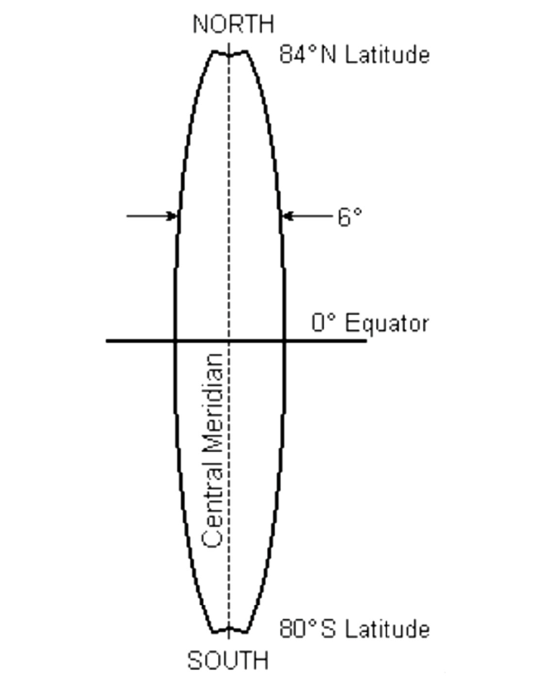
A common projection used in Canada is the Universal Transverse Mercator (UTM), which is also used by the Canada Centre for Mapping and Earth Observation (CCMEO) for the National Topographic System (NTS) maps (Natural Resources Canada, 2016). UTM is a conformal projection and is split into 60 individual projections (zones) of 6° longitudinal width, spanning from 80° S to 84° N, as shown in Figure 8.

While a geographic coordinate system is a spherical representation of positions described using angles from central lines of latitude and longitude, a projected coordinate system is a planar representation of positions described using x and y coordinates from a central x and y axis. The UTM projection uses its own central meridian from which to derive positions within its zone. UTM coordinates are measured in meters from each zone’s central meridian (Eastings) and the Equator (Northings). The central meridian is given a false Easting of 500000 m with values increasing from West to East, therefore eliminating negative numbers for the entire width of the zone. The Equator has a Northing of 0 m (for the Northern Hemisphere) increasing in value from South to North (U.S. Geological Survey, 1987).

Scale factors are ratios of the scale along meridians and parallels compared to a standard line of true scale. These scale factors determine the scale distortions for measurements on a projected surface. The central meridian in each UTM zone is given a constant scale factor of 0.9996, which was the value chosen in order to minimize scale variations within each zone. Since the scale factor increases with distance in the East and West directions, two vertical lines of true scale (1.0000) will be present, which occur roughly 180 km either side of the central meridian. The maximum variation in each zone reaches 1 part per 1000 (1 ppt) from true scale at the Equator (U.S. Geological Survey, 1987). A smaller UTM projection, such as the 3TM projection in Alberta, spans only 3° in longitudinal width with a constant scale factor of 0.9999 along its central meridian. Reducing the longitudinal width of a single UTM zone is necessary for reducing scale distortions, but presents a problem when describing spatial features that span more than one UTM zone.

Figure 9 is a contour plot showing the UTM scale factor as a function of latitude and longitude based on coordinates projected in NAD83 UTM zone 12 across Alberta and Saskatchewan. As you can see from the contour plot, the scale factor dramatically increases in magnitude for points that are located outside the zone in which they were projected.

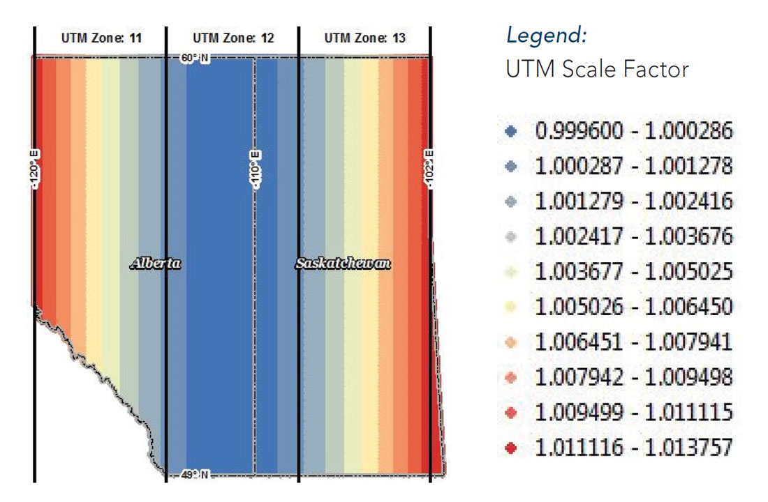
Consider a series of seismic lines located across Western Canada, projected in NAD83 UTM zone 12. A seismic line near the Alberta-Saskatchewan border at -110° E will be subject to projection distortion with an absolute scale factor of up to ~1.0003, which equates to 0.3 ppt. A seismic line near the Alberta-British Columbia border at -120° E, or near the Saskatchewan-Manitoba border at -102° E will be subject to distortion with an absolute scale factor of ~1.0138, which is two orders of magnitude larger at 13.8 ppt. Analyzing spatial data using an appropriate projection is therefore critical to minimizing scale factor errors.

Application

The term coordinate system refers literally to a system of coordinates, which in the context of this article is a unit of measure for determining locations relative to a reference frame. This should not be confused with the term coordinate reference system (CRS), which is used to describe a coordinate system, a datum, and optionally a projection, collectively. Many software applications allow users to specify a CRS (geographic or projected) rather than having to define a coordinate system, a datum, and a projection individually. The following sections identify some of the key factors when using coordinate systems, datums and projections in various applications.

Area of Interest

The area of interest is defined by the extent and coverage of spatial data, and each area of interest should be treated differently, whether global, regional, or local. A CRS that suitably represents individual areas of interest may reduce three-dimensional positioning errors and/or projection distortion errors as described earlier. Many different datasets covering many different areas of interest are often used collectively in a single geophysics project. For example, seismic data is often overlaid with global culture/basemap data, regional township grids, or local industry data in order to provide spatial context. Separating a large project into smaller areas of interest that can be defined by a specific CRS may improve the accuracy of results. Consider working with a geomatics/GIS professional to identify and create a suitable CRS for a specific project area.

Transformation Method

Transformations are required whenever there is a datum difference between the data source and destination. For example, an application might be using a CRS with a NAD27 datum, but the data might be using a CRS with a NAD83 datum. As mentioned earlier, the differences between NAD27 and NAD83 datums can lead to significant positioning errors, so a method is required to transform the CRS parameters of the source to match the CRS parameters of the destination. Using the appropriate transformation method ensures positional integrity, but – like the CRS – there are many transformation methods to choose from. NAD_1927_To_NAD_1983_CSRS uses a different transformation method than NAD_1927_To_NAD_1983_NADCON and NAD_1927_ To_NAD_1983_NTv2_Canada. Many software applications will try to perform the transformation automatically, but using the default method can be dangerous. In some cases a transformation must be applied to spatial data before it can be used, especially when the transformation method is either obscured or not possible within the software application itself (Berls, n.d.). If a custom CRS is used in an application, then a custom transformation may also be required in order to transform the data appropriately.

Data Acquisition

Survey monument coordinates in the Dominion Land Survey (DLS) system are typically established with respect to NAD83, and are geo-referenced using a combination of Precise Point Positioning (PPP), Global Navigation Satellite System (GNSS), and/or Real-Time Kinematic (RTK) network corrections, to name a few (Surveyor General Branch, 2014). Any spatial data acquired with reference to DLS monuments must therefore be transformed if the desired CRS is different from NAD83. Many survey companies will perform this transformation on a clients’ behalf (e.g. from NAD83 to NAD27), but not all spatial data is acquired and delivered in the same way, so close attention must be paid to ensure which CRS is being used.

Conclusion

There are no explicit rules regarding the collection, analysis and interpretation of spatial data for geophysical exploration, but understanding the theory behind datums and projections provides an awareness of the limitations and impacts that occur from decisions surrounding location accuracy. A coordinate system is meaningless without a datum, and a projection will always be subject to distortion, but using an appropriate CRS to represent the datum, coordinate system, and/or projection is impossible without knowing how the data was collected, what area of interest it covers, and how the data will be used. Uninformed decisions can lead to inaccurate interpretation and undesired results, potentially leading to financial, legal, regulatory, and environmental implications.

Acknowledgements

I would like to thank Brady Troyer, P.Eng., Mark Dumka, P.Eng., Dr. Steve Jensen, P.Geoph., and Nicole Willson, P.Geoph. for their input, advice, and feedback on putting this article together.