Denoising data is the essence of discovery. Raw seismic data are a jumbled collection of bits bearing little resemblance to geology. All of the steps in the seismic data processing workflow, including deconvolution, migration, and stacking are noise reduction techniques designed by geophysicists to highlight a certain type of signal hidden in the noise that is seismic.
The method introduced in this article suggests a flexible, extensible collection of processing steps for use with seismic (or other) data. Using a simple image translation network, this research removed white noise from a seismic section. The methodology is applicable to the removal of incoherent noise (white, Gaussian, flicker, etc), coherent noise (multiples, ground roll, air wave, etc), and wave propagation effects (migration, deconvolution, stacking, etc).
More succinctly, image translation networks can be used to replace seismic processing in its entirety.
Unfortunately, without a large variety of training data, image translation will fail to generalize to new data, and the algorithm will appear to have failed. This is because the training data doesn’t span the full input domain, and thus the output domain is limited in extent. Incorporating more training data which is varied in geophysical scope will solve this problem. This is not a trivial problem, however, as most seismic data is held proprietary.
A Note on Reproducibility
All the data and code referenced in this article is located in a public repository [1]; it’s free to modify and/or use for research or commerce.
The real seismic data used in this research was a small section of the Teapot Dome filtered, migrated 3D data volume. It was obtained via the SEG open data repository [2]. Thanks to ROMTOC and the U.S. Department of Energy [3] for providing the Teapot Dome dataset.
Algorithm Selection
The image translation network used in this research was a pix2pix network, designed by Phillip Isola, et. al [4]. It utilizes a supervised learning approach to image translation, wherein the training data are identical clean data – noisy data image pairs. This is powerful only insofar as users have access to identical pairs. There is another image translation architecture, called UNIT, designed by Ming-Yu Liu, et. al [5] which utilizes an unsupervised (or semi-supervised) approach to image translation. The UNIT architecture relaxes the identical data pair constraint and is thus applicable to a greater variety of problems.
The pix2pix network is a generative machine learning algorithm. Based on Alec Radford, et. al’s DCGAN [6] architecture, the pix2pix network learns image representations in its latent space, and once trained, can be used to generate unique images.
A GAN is a Generative Adversarial Network [7] in which one learning algorithm competes against another in a minimax optimization setting.
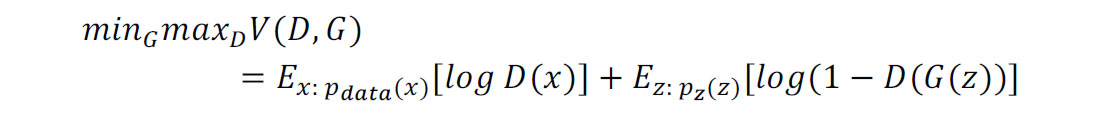
The first learner, called the generator (G above), is optimized to generate images which resemble input images. The input to the generator, z, is simply a noise tensor. The second learner, called the discriminator (D above), is optimized to distinguish between real images (from the input set, called x above) and false images (generated by the generator).
The effect is that, as training progresses, the generator network generates images of increasing similarity to the input set, and the discriminator distinguishes these generated images with increasing accuracy. When some stability threshold is reached, or early stopping occurs, the discriminator is chopped off the back of the network, and the standalone generator is used to create images which are of the same characteristics as the input space.
A conditional GAN [8] is a standard Generative Adversarial Network, except that an additional prior (that is, another known piece of information) is input into both the generator and discriminator, forcing the network to converge towards output which is similar to the additional prior, in our case an image.

As we can see in the equation above, the notable difference between a conditional GAN and an unconditional GAN is the additional prior, y, input into the network. This additional information “conditions” the error surface towards extrema in regions local to similar dimensionality.
Both unconditional and conditional GANs can be designed with a variety of generator and discriminator networks, though many use neural network architecture. These systems can thus be used to generate data including any data type. For example, it’s possible to design GANs to generate word embeddings, music, text, and images. The pix2pix image translation network is a special case of a conditional GAN which uses image data as its prior.
In the case of this research, both the generator and discriminator networks used conditioning. The noise added to generate stochasticity in the results is added through dropout layers rather than an additional Gaussian noise vector input. This work also utilized the L1 regularization parameter discussed in the Isola article (ref. 4). An L1 regularizer is used in the loss function to stabilize convergence to a global minimum; GANs are notoriously unstable, as seen (in the case of L2 regularizers) in the form of blurry output images. The generator was an encoder-decoder network with skip connections between its mirrored layers (Unet), and the discriminator was a basic three-layer convolutional neural network (CNN).
Results
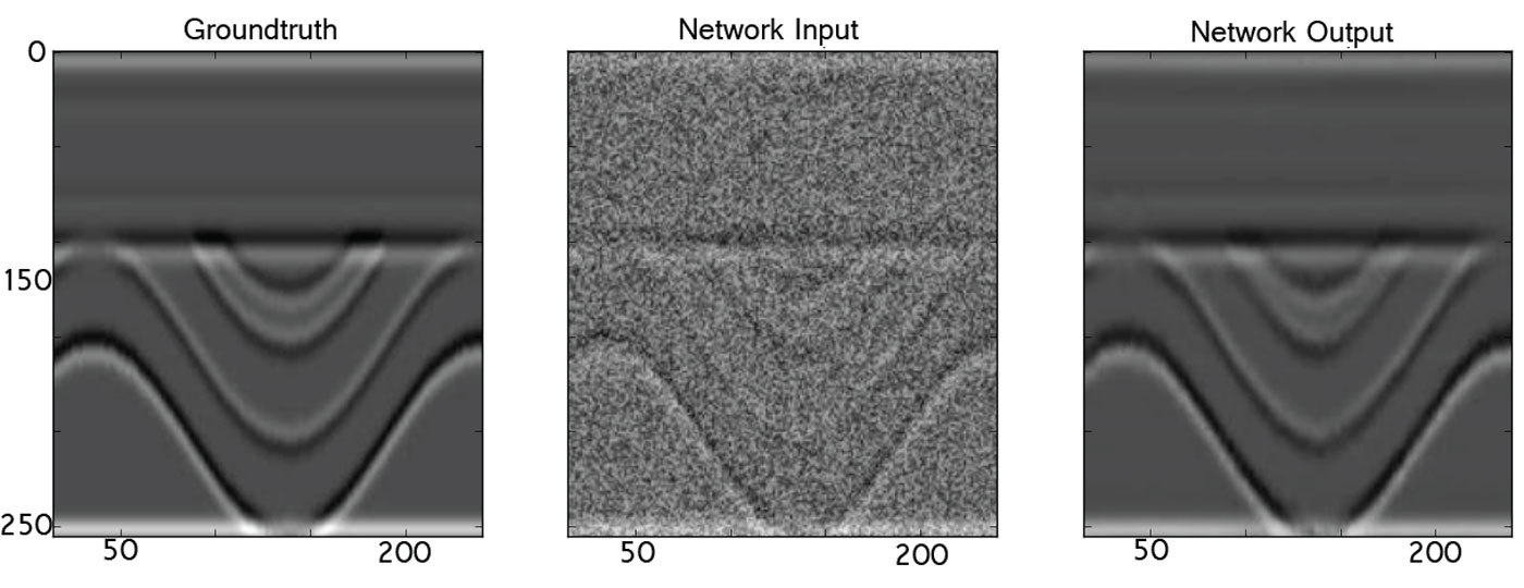
When operating on synthetic data, the pix2pix network outputs beautifully reconstructed seismic sections. As is shown in figure 1, the input section has noise on the order of 2.6 decibels loss but the output has loss on the order of 0.2 decibels. This behavior is to be expected since the training data pairs were all constructed using the same wavelet and similar acoustic impedance boundary distributions.
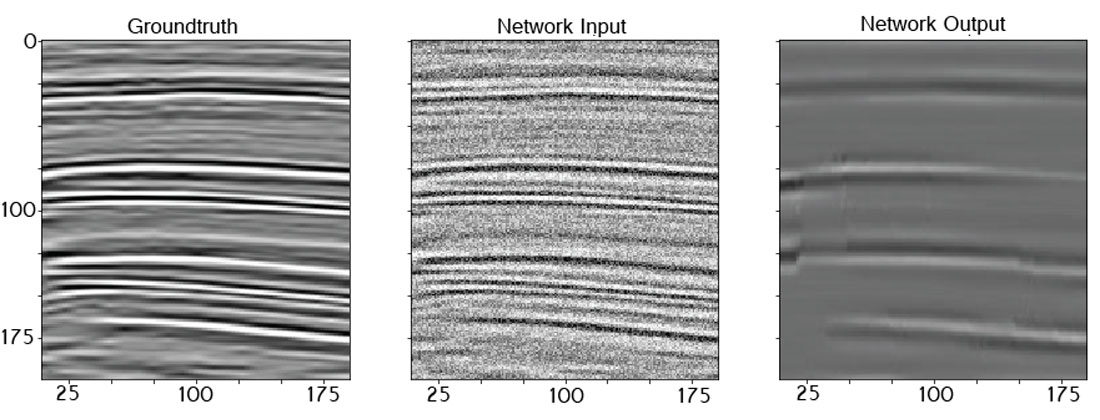
To reiterate, this seismic section was not shown to the pix2pix network during training. Though the pix2pix network has generalized to operate on this unseen (blind) data, its accuracy is significantly reduced when operating on data of increased apparent frequency, non-stationarity, or alternative noise pollution. In the face of real data, the pix2pix network does not output the same convincing results. Figure 2 shows these results.
When compared to three common image denoising strategies on the basis of L1 loss, the image translation pix2pix network performs significantly better on the synthetic data examples, and significantly worse on the real data examples. For the uninitiated, the L1 loss is similar to the L2 loss:

except the second-degree norm is replaced with the first-degree norm:

The alternative denoising strategies tested against the image translation network included total-variation filtering, bilateral filtering, and wavelet transform filtering.
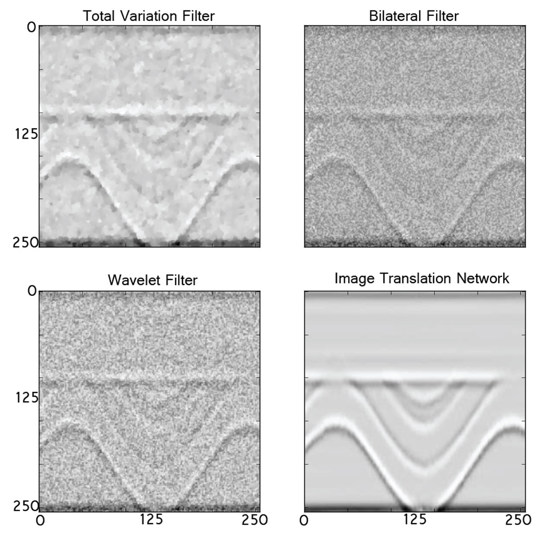
Figure 3 shows the denoising algorithm comparison on the same input data shown in figure 1. The average L1 loss calculated across the entire blind testing set is shown in table 1.
| L1 Loss Mean Value | Standard Deviation | |
|---|---|---|
| Table 1. Loss results from various image denoising techniques. | ||
| Pix2pix network | 2059.9 | 1456.6 |
| Total variation filtering | 4909.5 | 1996.2 |
| Bilateral filtering | 5657.3 | 1629.8 |
| Wavelet filtering | 6167.8 | 1365.8 |
With respect to the pix2pix network loss, the average increases in loss with the conventional methods were: TV filter – 3.8 dB, bilat filter – 4.4 dB, wavelet filter – 4.8 dB. The losses over the blind testing set are shown in figure 4. This highlights the accuracy of the pix2pix network on the synthetic data samples.
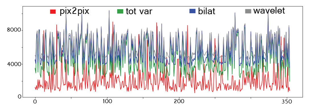
The real data denoising strategy comparison is shown in figure 5. As noted, the image translation network performs at a significantly lower accuracy than the conventional methods.
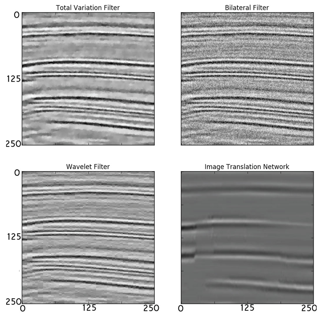
On the real data, with respect to the pix2pix network loss, the decreases in loss with the conventional methods were: TV filter – 2.2 dB, bilat filter – 2.0 dB, wavelet filter – 3.1 dB.
Algorithm Flexibility
The above results are indicative of an algorithm which is overfitting. The reason this image translation network is overfitting is that, again, the input training pairs didn’t span the full dimensionality of the input space. The algorithm does work, and is more accurate than conventional means when used on data it’s familiar with. However, to make a commercially viable network a user would need to train with data corresponding to real seismic. I urge the interested reader to download the Teapot Dome dataset, slice it into panels, generate training pairs by adding noise, and train the network. Once this is done, the network will perform at a level capable of operating commercially.
I also remind the reader that this code can be used to remove other wavefield artifacts. Train the pix2pix network on pairs of primary-energyonly- shot-gathers vs. multiple-and-primary-energy-shot-gathers, and you’ve just built a system to remove multiples from seismic. Train the pix2pix network on pairs of unmigrated images vs. migrated images, and you’ve just build a system which performs migration.
The code used in this research utilized a 2D – 2D mapping. It’s entirely possible, though non-trivial, to build a system which maps data from one dimensionality to another. For example, if you change the input and output layers of the discriminator and the generator networks to translate data from 5D to 3D, you could build a system which takes completely raw field seismic, and outputs a migrated, stacked volume, ready for interpretation.
Generative data translation networks are relatively new, and thus are relatively underexplored. We’ve seen that adequate training data is imperative to building successful systems, but if that constraint can be fulfilled, it’s possible to use these ideas to build platforms to solve problems which conventionally take months (seismic processing) in milliseconds.

Related Reading


Join the Conversation
Interested in starting, or contributing to a conversation about an article or issue of the RECORDER? Join our CSEG LinkedIn Group.
Share This Article