Dimensionless Gradients Applied To Pore Pressure Prediction – A New Standard

Given the cost of controlling problems associated with drilling pore pressure surprises, it is important to develop concise methods for predicting pressure gradients ahead of the bit. This paper sets out a new standard for working with gradients and explores the Eaton relationship between gradients and seismic velocity. A main point is that pressure prediction methods are simplified greatly if pore pressure, overburden stress, and mud weight are all expressed as a gradient in the same set of units. To demonstrate, we show examples from real drilling situations.

Interval and Average Gradients

Interval gradient, G_i, is equal to the difference between two pressure measurements divided by interval thickness. An analogy is interval velocity equal to thickness divided by the difference between two time measurements. Average gradient, G, is pore pressure divided by depth, D, where D is defined explicitly as TVD-KB i.e. true-vertical depth from derrick floor. An analogy is average seismic velocity.

The units for gradients are force (weight) per unit volume. To keep the following equations free of conversion factors and dimensionless as possible we express all gradients in the same units as mud weight as either kilograms per cubic meter (kg/m³), pounds per gallon (ppg), or specific gravity. In this text we use pressure gradient and density interchangeably (i.e. we assume a standard gravitational constant).

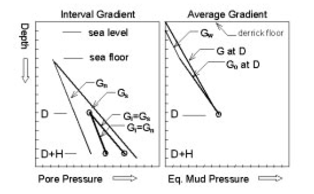
Confusion between Gand G_i is understandable. As illustrated in Figure 1, G is the static mud weight that balances formation pore pressure at depth D, that is, G is equivalent mud weight. G_i, on the other hand, is a physical property that, for permeable intervals, is equal to formation fluid density. While G_i can be constant for long intervals, G varies continually with depth. As given in Figure 1, G at depth (D+H) equals (GD+G_iH)/(H+D). A more concise form of the relationship is:

The equation illustrates an important attribute. Delta is positive for G_i>G and negative for G_i<G. To describe the equation differently, G is a known (equivalent) mud weight at depth D determined from a kick, estimated from seismic or wireline acoustic data, or derived from a direct measurement (e.g. from a repeat formation tester). Delta is the incremental increase in mud weight needed to drill to depth (D+H) or, when Delta is negative, Delta is the added overbalance at depth D+H if mud weight cannot be decreased.

Now consider three additional gradients G_s, G_n, and Gowhere G_s is the average sediment density between the sea floor and depth D, G_n is the average formation water density between the sea floor and depth D, and G_o is the average pressure gradient between the sea floor and D. We define the new term, G_o, to better describe the relationship between gradients and seismic velocity in deepwater situations. The relationship between G and G_o is given by:

where A is air gap (height of the derrick floor), G_A is air gradient (usually assumed zero), G_W is sea water gradient, W is water depth and D_BSF is depth below sea floor. G is an artificial property that decreases as A or W increases. G_o is a real property that is independent of W or A. As a reference to terms used in the literature, lithostatic and hydrostatic pressure gradients (i.e. lithostat and hydrostat) are somewhat ambiguous terms used to reference G_s and G_n to sea level or derrick floor or, in some cases, to the sea floor.

Velocity-Derived Gradients

Vertical effective stress is equal to (G_s-G_o)D_BSF and mean effective stress, for transverse isotropic conditions, is equal to (G_s- G_o)(D_BSF)(1+2k)/3 where k is the horizontal to vertical effective stress ratio. Porosity and velocity in mudstones are functions of effective stress and are independent of water depth. From the Eaton relation the ratio of effective stress at two stress states is a power law function of the ratio of acoustic velocities at the two states. If one stress state is (G_s-G_n) and k is a rock property that does not vary with G, the Eaton relation can be expressed as:

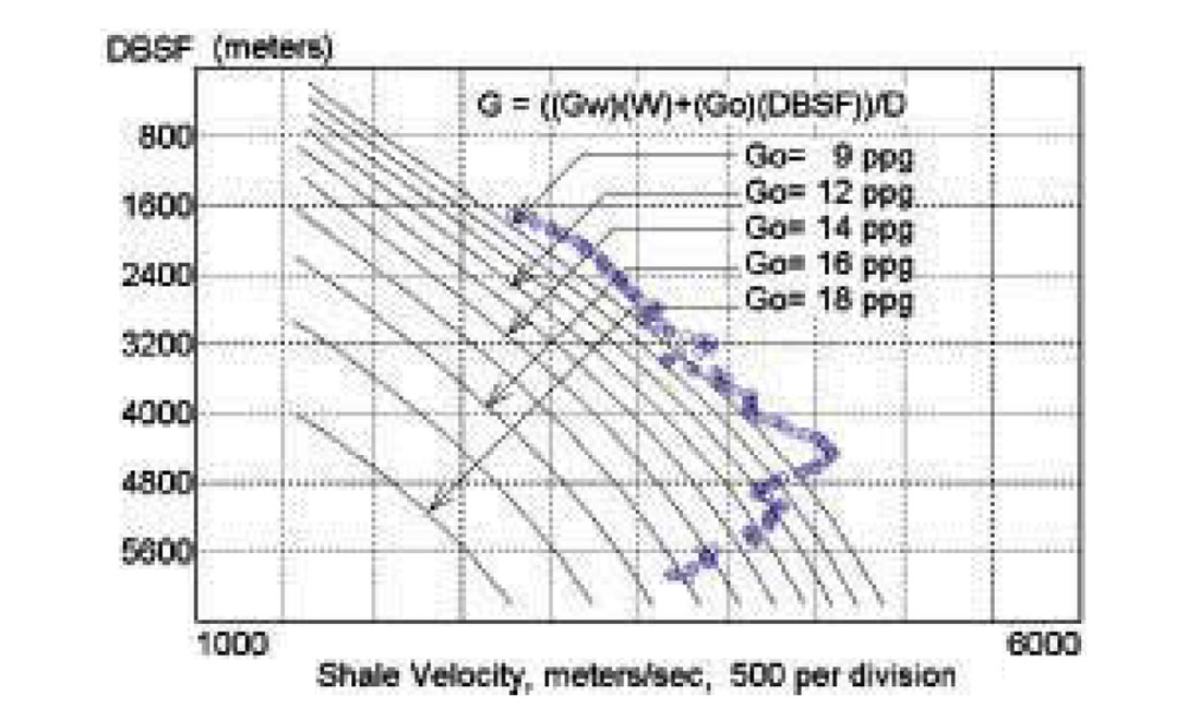
where V is seismic interval velocity and V_n is interval velocity at the same depth if pore pressure is normal. The determination of V_n is complex and not included in the scope of this paper but we do include a graphical solution of the Eaton relation in Figure 2 that uses a global V_n function.

The Eaton relation is commonly used for deriving pore pressure gradients but it does not come without controversy. One can argue that the right term of the equation is expressed more correctly as

where V_ma is matrix velocity. One can also argue that the two G_s terms in the equation are not equal as is generally assumed. For example G_s in the numerator is present day average sediment density and G_s in the denominator is average sediment density if pore pressure is normal.

Now consider three examples (the situations are real but the values have been rounded to make the concepts more clear). The main challenge in the examples is the selection of G_i. For intervals that are a single hydraulic compartment, use G_i equal to 228 kg/m³ (1.9 ppg) for gas bearing intervals and 1060 kg/m³ (8.9 ppg) for water bearing intervals. For intervals that are isolated cells interbedded in massive overpressured mudstone, assume G_i equals G_s. If G_s is not known, use a value for G_s of 2310 kg/m³ (19.25 ppg). In practice G_i is derived from equations of state as a function of temperature and pressure and G_s is derived from density log data, acoustic transforms, or compaction models.

Example 1

A well in the Gulf of Mexico took a minor kick at a depth of 3657 TVD-KB and needed a mud weight of 1680 kg/m³ (14 ppg) to balance pore pressure. What mud weight will be needed 200 depth units ahead of the bit? We purposely do not specify meters or feet because the equations are dimensionless.

The first part of the solution is the estimation of interval gradient. From local knowledge we assume massive shale with isolated sandstone intervals and use a value of G_i equal to G_s or about 2310 kg/m³ (19.25 ppg). From Equation 1, Delta is (2310- 1680)(200)/(3657+200) or about 33 kg/m³. In ppg units Delta is (19.25-14)(200)/(3657+200) or about 0.3 ppg and G at (D+H) is 1713 kg/m³ (14.3 ppg).

Example 2

A well in Michigan will penetrate a gas bearing pinnacle reef at a depth of 7,000 feet. What mud weight is required to drill the reservoir? We know that the gas-water contact is at 8,000 feet and that the aquifer is normally pressured. We also know that the formation water is salt saturated and has a weight of 1200 kg/m³ (10 ppg).

The first step is easier than Example 1. G_i is 228 kg/m³ (1.9 ppg) for gas. G is 1200 kg/m³ (10 ppg) at the contact at 8000 feet (D in the equation is 8000 feet). For this case, where D>(D+H), H is negative and equals -1000 feet. From Equation 1, Delta is 139 kg/m³ (1.16 pg). The mud weight required to drill the reservoir is 1339 kg/m³ (11.16 ppg).

Example 3

An exploration well is planned in the North Sea. What mud weight will be needed to drill to a depth of 4050 meters below sea level if the seismic velocity is 3000 meters/second for the mudstone interval from 3600 to 4000 meters? Water depth is 50 meters.

From Figure 2, G_o is 15 ppg (1800 kg/m³) for a velocity of 3000 meters/second and D_BSF of 4000 meters (i.e. 4050-W). From Equation 2, the equivalent mud weight, G, is only slightly less than G_o and the required mud weight to reach total depth is therefore about 1800 kg/m³ (15 ppg).

As a best practice we would normally determine G_o at the mid-point of the interval (3600+4000)/2, and project from the mid-point depth to total depth with Equation 1. Also, in practice, we would normally look at other methods to verify the seismic prediction. For example, if we use the known top of overpressures in this region at 1050 meters and assume G_i equals G_s from 1050 to total depth, Equation 1 would project to a value of 1990 kg/m³ (16.6 ppg).

Conclusions

As a summary consider the following epilogue to the above examples. The Gulf of Mexico well continued to drill with a 1680 kg/m³ (14 ppg) mud weight and took a $4 million kick at a depth 200 meters below the first kick. Post-well appraisal indicated that the small increase in mud weight predicted in the above solution would have prevented the problem.

For the well in Michigan the operator smartly drilled into the reservoir with 1344 kg/m³ (11.5 ppg) mud weight (slightly overbalanced for safety) and continued to drill with that mud weight to maintain control at the top of the reservoir. As G decreased with increasing depth (because G_i<G), the fracture gradient correspondingly decreased. At some point the well lost returns due to fracturing and the mud pressure dropped. The well blew out and burned.

For the North Sea case, the well was drilled to about 3800 meters with a maximum mud weight of 1800 kg/m³ (15 ppg). At that point it was observed that the formation tops were coming in shallow to prognosis indicating that the seismic velocity used in the depth conversion was likely too fast and, therefore, that the pore pressure prediction was likely too low. To get a new estimate of velocity, a drill-pipe derived interval thickness (between two horizons identifiable both on seismic and in drill cuttings) was divided by a seismic-derived time difference for the interval. This gave a new estimate of pore pressure gradient. Mud weight was increased to 1920 kg/m³ (16 ppg) and drilling continued without incident. A repeat-formation-tester measurement verified the new prediction and the savings attributed to the real-time adjustment, that avoided a well control problem, was $3 million.

Acknowledgements

We thank BP for sponsorship and we particularly thank the many participants of ChevronTexaco/BP Alliance pore pressure courses for constructive feedback on the methods set out in this text. We also acknowledge Neil Goulty for his constructive comments and Bob Bruce for suggesting that pore pressure can be usefully expressed as a gradient.