Discovering A Supermodel – A Rock-Physics Tutorial

Quantitative interpretation (QI) involves making predictions of rock and fluid properties from seismic amplitudes. Within the QI workflow, a number of components can greatly benefit from rock physics, which itself is an incredibly diverse field. Rock physics covers the measurement of rock properties in the lab, the empirical and theoretical relationships used to predict elastic properties from geological parameters, and the analysis of elastic properties derived from well-log and seismic data. Prediction of elastic properties is of particular interest, as these predicted properties can be used to generate synthetics, synthesize well logs, or create rock-physics templates for interpreting crossplots of inversion attributes.

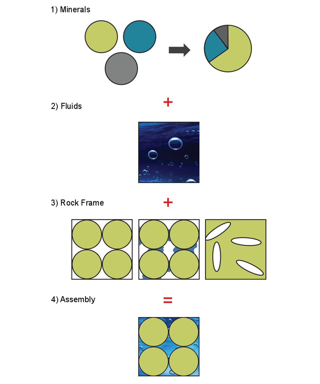
In this tutorial, I explain the four steps required to create models of saturated reservoir rocks with different fluids and lithologies (Figure 1):

1. Modelling the minerals
2. Modelling the fluids
3. Modelling the rock frame
4. Assembling the components

The aim of a rock-physics model is to predict elastic properties (velocity, impedance, moduli, etc.) for different geological scenarios. The specific properties being predicted – elastic moduli, attenuation, anisotropic parameters – depend on the application at hand, but the common aim is to understand the behaviour of rocks in different exploration and production cases. Here, I explain simply how different components fit together to produce a geologically relevant rock model, and point out where different Canadian geologies require specific considerations within the modelling process. All relevant equations are contained in the references provided, but are omitted here to focus on the overall process. This paper is an expansion of an extended abstract from the 2015 GeoConvention (Reine, 2015) and some of the examples have been previously shown (Reine, 2016).

Motivation

A simple example of how rock-physics modelling can be used for QI puts the process into context. QI often involves crossplotting the seismic attributes obtained through AVO inversion. Different clusters or trends of data can be interpreted, or classified, based on similar behaviour of well logs. But what if the well data is limited in its geological scope? Figure 2a shows a crossplot of Mu-Rho (μρ) vs. density (ρ), commonly used to classify the McMurray Formation. This one well encountered a thick sand interval, as evidenced by the point colour, which corresponds to the logged gamma-ray values. But surely the seismic will cover areas in which the McMurray is muddy. What is the basis for deciding whether an equivalent seismic crossplot is showing mud rather than sand? This lack of information often leads to the interpretation philosophy of "different is bad", which is far from the quantitative nature of QI that we are trying to achieve.

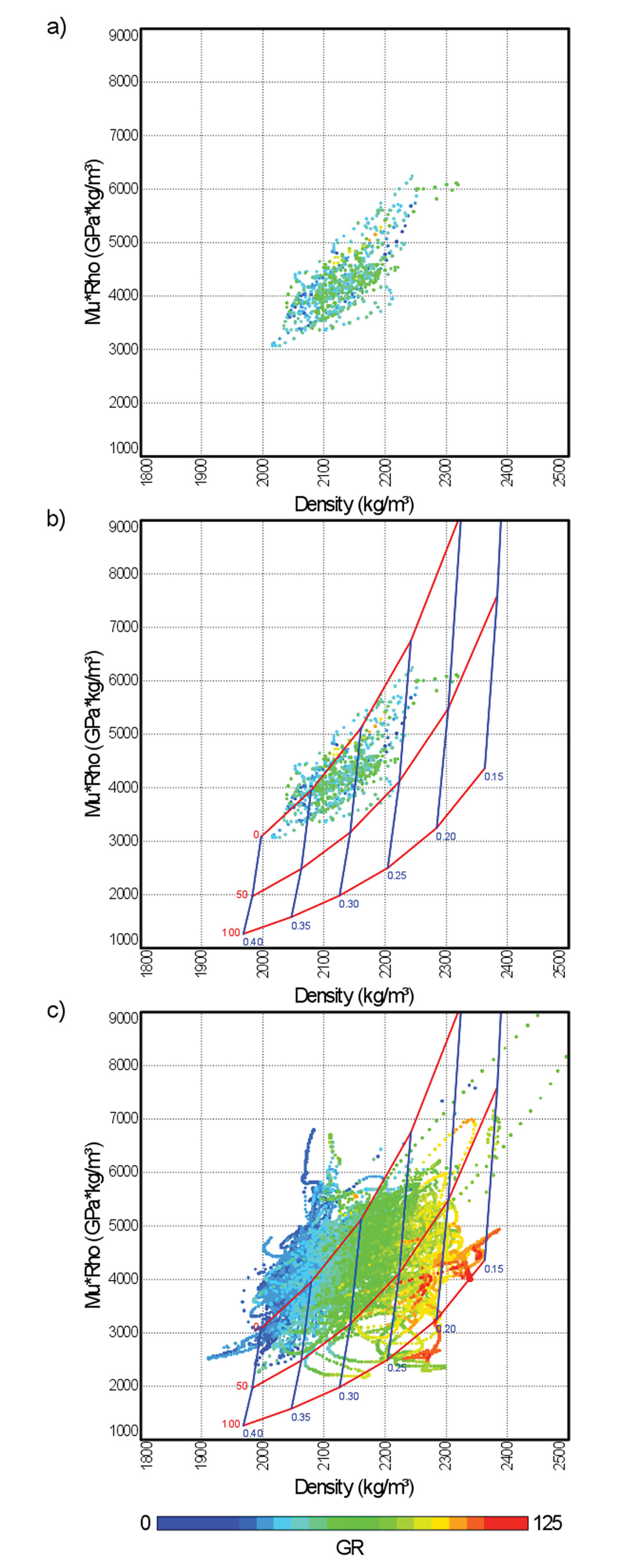
Using rock-physics modelling, it is possible to construct a template that honours the data we know and extends the interpretation to situations that we don't know. Figure 2b shows model calculations for 0%, 50%, and 100% clay content (red lines), with porosity varying from 15% to 40% (blue lines). The resulting template provides a basis for interpreting lithology should seismic data fall in regions of the crossplot that are different from the sandy well. Figure 2c shows data from fifteen wells with a range of geology. The data with higher gamma-ray values are seen to plot in the template region suggesting higher clay content and lower porosity than the clean sands, confirming the usefulness of the template.

Minerals

The first step in the modelling process is to determine the mineral properties. Mineral changes can be used to model different lithologies or depositional environments. In the example that was shown in Figure 2, the models that varied from sand to mud were based on changes in the mineral properties. Identifying these types of changes in the subsurface has obvious uses in well planning and resource estimation.

The mineral bulk modulus, shear modulus, and density are measured in the lab, and this data is not often available on a field-by-field basis. Some minerals, such as quartz, have elastic properties that are very consistent from field to field, while other minerals, most notably clays, are substantially more difficult to quantify. Fortunately, a number of researchers have summarized published measurements. Mavko et al. (1998), for instance, tabulate dozens of different minerals from just as many sources, and Avseth et al. (2005) provide a similar table for the properties of clay minerals. The bulk and shear moduli of some common minerals are shown in Figure 3.

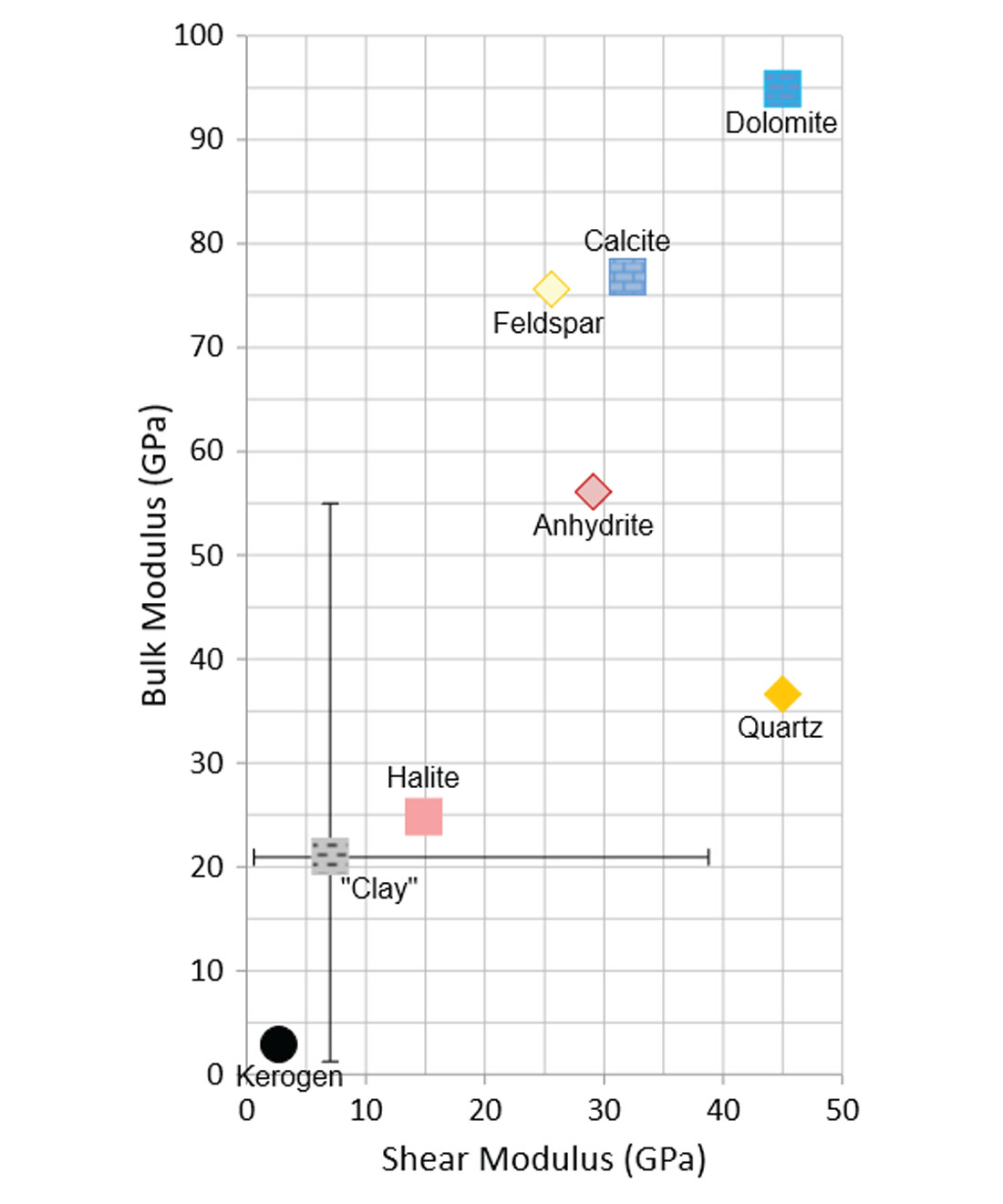
The mineral grains are the building blocks of the rock-physics model. For most minerals, there is a direct correspondence between the measurements made on a single mineral crystal and the properties of the grains. For clay minerals, however, the rock building blocks are not simply scaled-up crystals. Clay particles consist of layered clay minerals, such as kaolinite, and bound water. This arrangement makes for grains that are much less stiff than the individual minerals. Although some tabulated results are based on measurements of these larger particles, often the clay properties must be calibrated with well data in the modelling process. The error bars for the clay point in Figure 3 cover the range of values for different clay minerals and composite particles given in published results.

For a single-mineral rock, searching tables of measurements is all that is required for the mineral properties step. For the more realistic situation in which a variety of minerals are present, a set of effective mineral properties must be determined. Knowing the fractions of the minerals, from x-ray diffraction (XRD) data, x-ray fluorescence (XRF) data, or log analysis, is therefore an important piece of information. While digital rock physics can use the mineral fractions and their exact distributions to calculate models, this is extremely complex, and it is much more common to model the rock with an "effective" grain composition.

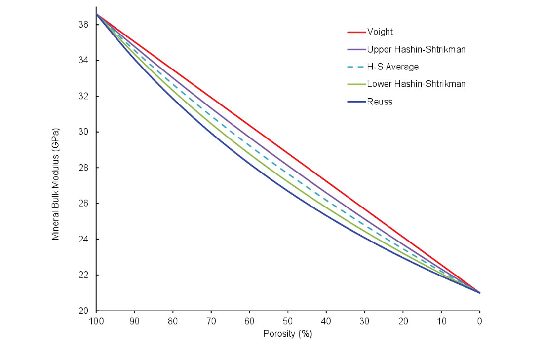
For an effective mineralogy, bounds and averages are used to compensate for not knowing how the grains are arranged. Figure 4 shows a number of bounds for a mixture of quartz and clay. When the elastic properties of the different minerals in the mixture are similar, these bounds are close in value, and for most situations an average of the upper and lower bound is sufficient. Other situations make using an upper (stiff) or lower (soft) bound more appropriate than an average (Avseth et al., 2005). Certain shales are examples of where a soft bound could be used, where the rock is clay-dominated with suspended quartz grains. A summary of different bounds is given by Mavko et al. (1998), with the upper and lower Hashin-Shtrikman bounds being commonly used.

Fluids

The economic appeal of fluid modelling is intuitive; locating gas vs. water, measuring the extent of a steam chamber, and detecting pressure drops by the presence of free gas are all fluid-modelling scenarios. While it has become commonly known that gas causes a decrease in velocity compared to brine or oil, it is also possible to quantify these effects more generally. Determining the fluid properties is the second step in the rock-modelling process.

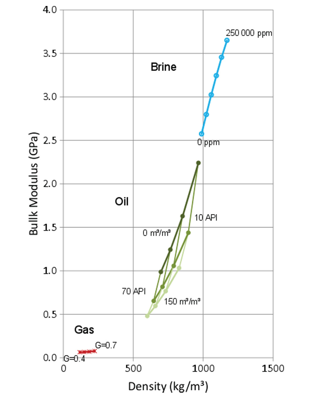
Fluid density and moduli are typically calculated using empirical relationships such as the well-known Batzle-Wang equations (Batzle & Wang, 1992), and subsequent expansions of that work (Han and Batzle, 2000a,b). These equations describe how the elastic properties of fluids are affected by reservoir temperature and pressure, and by specific parameters for each phase. These parameters include the specific gravity of the gas, the API and gas-oil ratio of the oil, and the salinity of the brine. Frequently, these values are well known for a field, due to their use in engineering and for determining the economic value of the resource.

Figure 5 shows the relative density and bulk modulus for gas, oil, and brine over a range of fluid properties at a specific temperature and pressure. As expected, gas has the lowest density and is the most compressible. Interestingly, heavy oils (low API) with only small amounts of dissolved gas are similar in properties to fresh water. This is a situation encountered in Alberta's oil sands, although another elastic property can be used to make the distinction between the two.

The shear modulus of fluids is generally near zero; however, heavy oil violates this behaviour. Batzle et al. (2006) discuss the shear properties of heavy oils, which have been measured as a function of temperature and frequency of investigation (Behura et al., 2007; Rodrigues & Batzle, 2015; Spencer, 2013). In general, the properties of heavy oils do not follow the Batzle-Wang relationships very well, and other models are needed (e.g. Han et al., 2014).

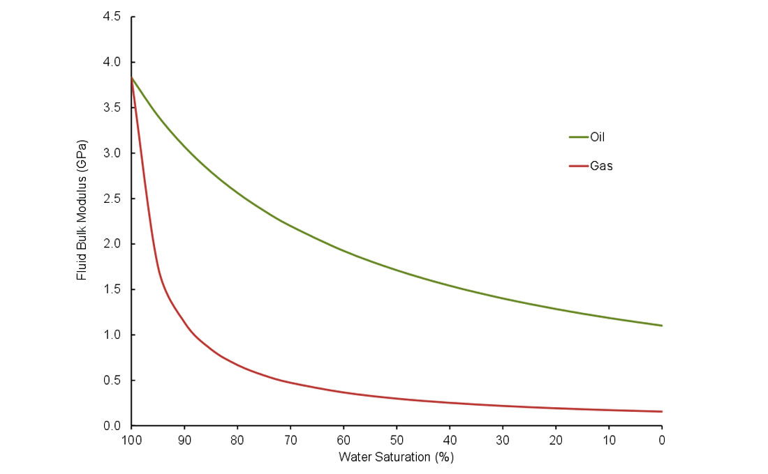
The elastic properties of the effective fluid are taken as a Reuss average of the three phases when the fluids are assumed to be uniformly saturated. If this is not the case, for example in some cases of water injection or gas dissolution, a patchy saturation model must be used when assembling the model components (Mavko et al., 1998). Patchy saturation also tends to be more representative for small saturation values. Figure 6 shows the effect on the fluid bulk modulus of increasing the hydrocarbon saturation for a uniform saturation.

Rock Frame

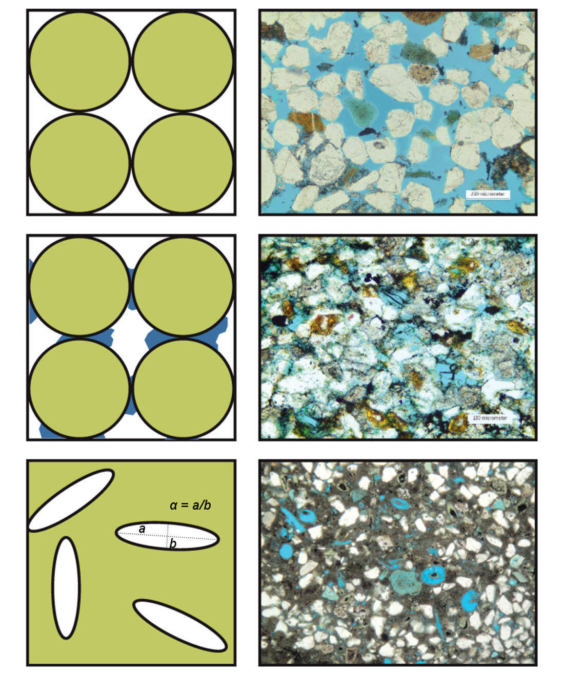
Many different approaches exist to model the stiffness of the rock frame itself. Known as the "dry" case, it is independent of fluid effects, and instead depends on how the rock is put together. Is the rock unconsolidated or cemented? Are the pores the result of grain packing, or are they due to cracks or dissolution? Many different models and situations are possible, but here I limit the discussion to the cases shown schematically in Figure 7. The utility of the rock-frame component is that it is possible to model different porosities or degrees of cementation, properties which are factors in resource recovery.

In unconsolidated rocks the elastic properties of the frame are determined for a packing of identical spherical grains (Dvorkin & Nur, 1996). The properties are therefore a function of how tightly packed the grains are, which in turn is a function of porosity, effective pressure, and the number of contacts per grain. Introducing even small amounts of cement can greatly increase the stiffness of a rock. Dvorkin and Nur (1996) also present a second model that describes this behaviour as a function of the cement's elastic properties and the amount of cement with respect to the grain distribution.

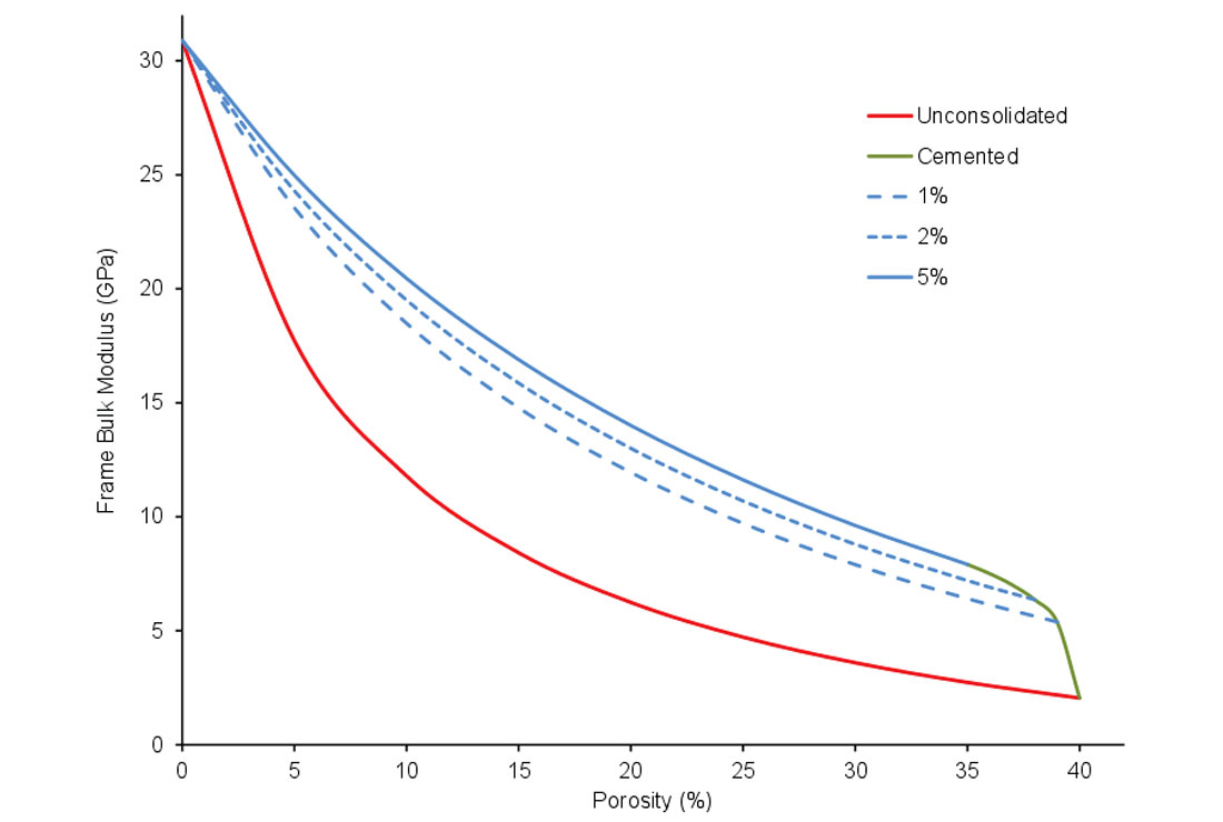
Because of the assumptions on the grain uniformity for the unconsolidated and cemented models, typically only the maximum porosity is modelled. The models for all other porosities between this maximum (critical) porosity and zero porosity (effective mineral state) are calculated using an interpolation between these two endmembers. For sandstones, the critical porosity, above which the grains are no longer in contact, is often around 40% (Nur et al., 1998). When clay minerals are present, this value can be lower.

The use of interpolation for intermediate porosities is heuristic; that is, it is logical but without solid theoretical justification. Nevertheless, it also fits well with experimental results. The type of interpolation is matched with the mechanism for reduction in porosity. For porosity changes due to changes in grain sorting, a lower Hashin-Shtrikman bound is typically used. For porosity changes due to diagenesis (compaction or larger cement volumes), an upper Hashin-Shtrikman bound is typically used. These choices are empirical, and some examples of data that justify the choice are given by Avseth et al. (2005). Figure 8 shows the bulk modulus for models of cemented and uncemented grains over a range of porosities.

Inclusion models present a third option for modelling the rock frame, and are often used for low-porosity rocks (Xu and White, 1995) or rocks with fractures or dissolution porosity, such as carbonates (Xu and Payne, 2009). These models use the theory of Kuster and Toksöz (1974), which adds the effects of inclusions (pores) to a background medium with known properties. For shaly sands, such as the Montney, this starts with a mineral mixture of sand and shale, to which is added low-aspect-ratio pores for the inter-shale porosity, and high-aspect-ratio pores for the inter-sand porosity. This type of modelling can also be used to see the effect of fractures on the rock properties. To do so, the background medium is simply set to be a rock-physics model created using one of the other methods.

Assembly

Now that each of the components has been evaluated, and their elastic properties have been calculated, the remaining step is to put them together and describe the saturated rock as a whole. This step accounts for the stiffening of the rock due to the increase in pore pressure from a seismic wave acting on the fluid, minerals, and frame together. While density is simply a porosity-weighted average of the fluid and mineral densities, the Gassmann equations (Gassmann, 1951; Mavko et al., 1998) are frequently used to calculate the saturated-rock moduli as a function of the three parts previously described.

Part of the popularity of the Gassmann equations is that they tend to work reasonably well, even when the underlying assumptions are violated. Smith et al. (2003) give an excellent summary of the underlying nature of the equations and some different fluid-substitution problems for which they can be used. Most often, the Gassmann equations are used to see the effects, on well logs, of changing from one fluid to another. This application still requires the fluid modelling and mineral modelling components described above, but the frame component remains constant, and thus cancels out. For building a rock-physics model from scratch, all three components are used.

Despite their robust nature, there are circumstances in which alternatives to the Gassmann equations must be considered. One of the assumptions of the equations is that the shear modulus of the rock remains unchanged due to the presence of the fluid. As mentioned previously, this is not the case for heavy oil and generalized equations (Ciz and Shapiro, 2007) must be used. Low-porosity rocks, where there is little communication between pores, also violate the Gassmann model. In these situations, the Kuster-Toksöz theory is better employed, using inclusions that are fluid-filled rather than dry. Also, fluid substitution in rocks composed of multiple mineral types, especially with large stiffness contrasts, is expected to be more accurate using equations that account for that inhomogeneity (Saxena et al., 2015).

Templates

Following the procedure to this point will have used a set of parameters to produce a single rock model. While this may help give confidence in the understanding of a specific rock type, the real potential of rock-physics modelling is the ability to systematically change parameters and investigate relevant scenarios. Defining elastic properties as a function of a geological change allows curves and grids to be defined in elastic-crossplot space, creating a rock-physics template, as was shown in Figure 2.

Rock-physics models are typically calculated in terms of bulk modulus, shear modulus, and density. However, the models and templates are not limited to these attributes. Depending on the desired crossplot attributes, elastic properties such as Young's modulus, Poisson's ratio, λρ, μρ, impedance (I_P, I_S), v_P:v_S, and other properties can be derived as desired.

Attributes for crossplot classification are usually chosen to maximize the separation of different classes of data, for example, separation between low-porosity and high-porosity reservoir.

Before calculating a rock-physics template, it is necessary to calibrate the model to existing log and core data. Typically this is done by modelling a range of porosities, and observing the match to the data on a velocity versus porosity crossplot (Figure 9). Adjusting individual parameters and recalculating the model gives a great understanding of the relative contribution from each element. More robust understanding of the effects from parameter uncertainty can be obtained through Monte Carlo error analysis.

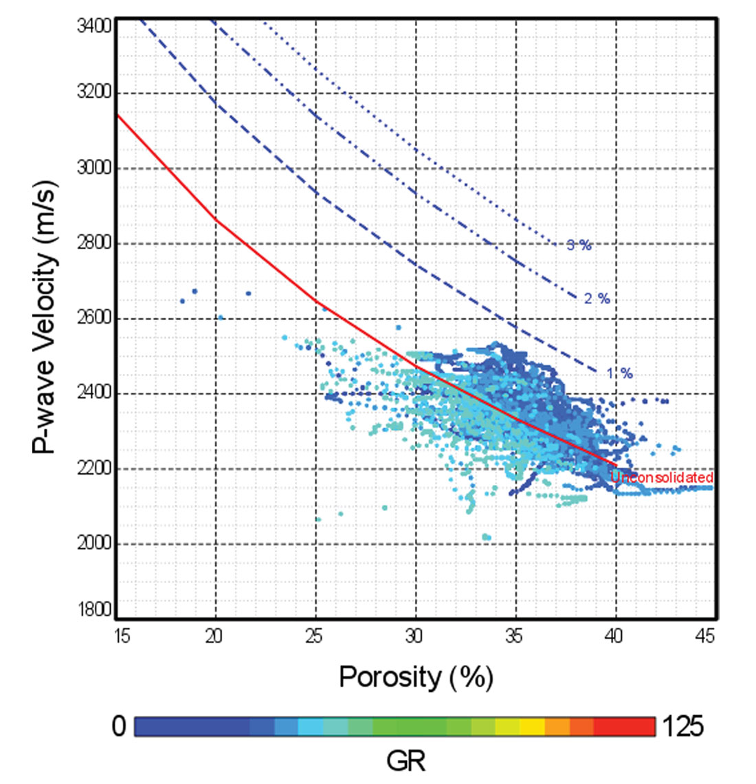
Calibration is best done using well data from an interval with well-known properties, for example, a water-saturated clean sandstone. Core measurements of porosity can be beneficial, as they tend to be more accurate than log-based measurements for mixed-mineral lithologies. The model is adjusted to reduce the mismatch between the predicted and modelled values. Mismatches can be caused by incorrectly assumed or measured parameters or an inappropriate model type for the rock, among other reasons. Once the known geological situation has been matched, the modelling can be extended to extrapolate undrilled situations that may be encountered by the seismic data.

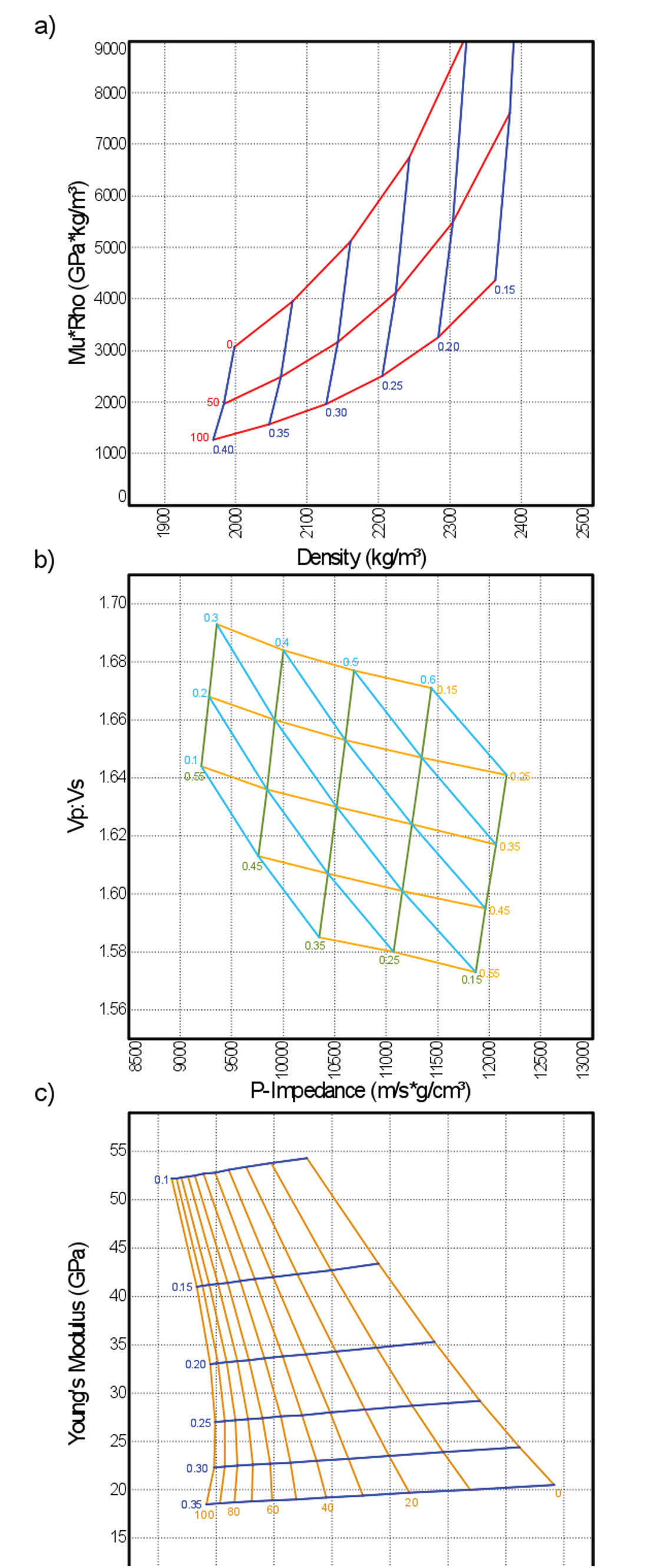
The template combination in Figure 2, variations in porosity and lithology, is not the only possible option for modelling. Modelling variables are determined by the expected conditions (lithology or fluid changes). In low-porosity resource plays, mineralogy can vary across the field while porosity stays relatively stable. In SAGD monitoring, fluids are variable as high-temperature steam and water replaces heavy oil. For a field that covers different depositional environments, the amount of cementation may vary as well. Figure 10 shows the templates for some of these scenarios. Once the templates are created, a final check can be performed to see if the trend of any available well data matches the template (Figure 2c).

Conclusions

Whether calculating inputs for a simple wedge model, predicting missing log data, or generating templates for crossplot interpretation, a rock-physics model is a valuable tool. Although there is a great volume of papers and textbooks to sort through, the process can be understood more simply in four stages: Modelling minerals, modelling fluids, modelling the frame, and assembling the components.

Combining a series of rock-physics models that cover a range of geological scenarios allows the creation of rock-physics templates. These templates are displayed on a crossplot of elastic properties along with the seismic data. This methodology allows the seismic data to be classified into geologically-meaningful categories, even in the absence of well data representing those groups.