Economics of Induced Seismicity: Trying to identify faults in the horizontal well planning stage

“Induced seismicity” refers to a seismic event that is caused by pore pressure and stress change associated with human activity (Boroumand and Maghsoudi, 2016). The maximum magnitude of induced earthquakes is smaller than what is seen with natural earthquakes (Metz et al., 2017); they tend to occur in swarms (Metz et al., 2017); and occur at shallower depths than natural earthquakes (Gomberg and Wolf, 1999; McNamara et al., 2015; Metz et al., 2017), which may explain why they have been reported to be felt at surface (Boroumand and Maghsoudi, 2016) though they are small in magnitude.

Induced seismicity affects not only the reputation of a company, but also the reputation of the industry, which has led the oil and gas Industry to take induced seismicity seriously and to try to address some of the public concerns (Chevron, 2017). Recognizing these concerns is reflected in the development of several regulatory enhancements as well as industry-led initiatives (Chevron, 2017).

Part of the solution to prevent induced seismicity may be to identify possible subtle faults within the seismic during the planning of the horizontal well, utilizing recent changes in seismic acquisition and processing such as:

1. Higher density seismic acquisition;
2. Depth imaging;
3. Diffraction imaging;
4. Frequency enhancement;
5. Noise attenuation to sharpen the edges of structural discontinuities;
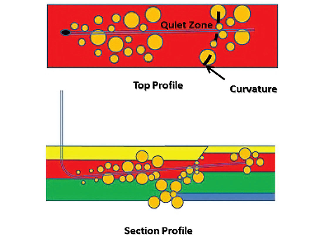
6. Structural attributes such as coherency; curvature; etc.

A byproduct from prestack depth migration is a better velocity field produced from the reflection tomography which utilizes a general ray-trace modeling-based approach (Bishop et al., 1985, Stork, 1992, Wang et al., 1995, Sayers et al., 2002; Satinder and Huffman, 2006) that improves the spatial resolution of the seismic velocity field (Sayers et al., 2002).

To further improve the tomographic velocities, one can employ automatic high density, high resolution, continuous (AHDHRC) residual velocities such as the ΔT program, that is essentially a reverse radon program where parabolas from the radon are fit to the data to determine γ that is utilized to correct the velocities; or, Swan’s (2001) Residual Velocity Indicator (RVI) that reduces the error within the gradient due to residual velocity (Spratt, 1987; Swan, 2001).

Traditional picked velocities are spatially coarsely sampled and the short wavelength variation in the stacking velocity field is lost (Suaudeau et al., 2002). This leads to poor stacking in areas where there are strong lateral variations in the seismic velocities and blurring of subtle faults. AHDHRC velocities increase the resolution and bring out subtle faults within the seismic by providing flatter gathers for stacking.

Overlaying tomographic or AHDHRC velocities over the seismic section illuminates the behaviour of the faults, such as whether it is leaky or a sealing fault (Kan and Swan, 2001) and it can bring out possible compartments within the geology that may affect production.

Introduction

“Induced seismicity” refers to a seismic event that is caused by pore pressure and stress change associated with human activity (Boroumand and Maghsoudi, 2016). These induced seismic events tend to be small in magnitude (0 < MW > 5.0). Events that are MW > 3.0 can be felt on the surface (BC Oil and Gas Commission, 2017).

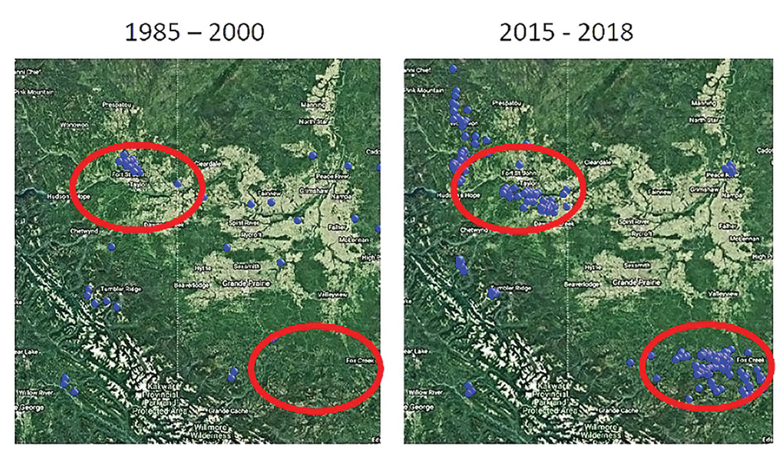
In January 2015 there was a swarm of earthquakes near Fox Creek, Alberta, which included a record-breaking tremor with a felt magnitude of 4.4. According to the Alberta Energy Regulator (AER) these earthquakes were consistent with being induced by hydraulic fracturing operations.

The maximum magnitude of induced earthquakes is smaller than what is seen with natural earthquakes (Metz et al., 2017); they tend to occur in swarms (Metz et al., 2017); and occur at shallower depths than natural earthquakes (Gomberg and Wolf, 1999; McNamara et al., 2015; Metz et al., 2017) which may explain why they have been reported to be felt at surface (Boroumand and Maghsoudi, 2016) though they are small in magnitude The biggest concern is induced earthquakes may trigger larger earthquakes on known or unknown faults (McGarr et al., 2015; Metz et al., 2017).

Understanding of faults in the area may be important for a couple of reasons:

1. To identify possible faults that may be reactivated during fracking;
2. Identify possible faults that may act to deviate the fluids and proppant used in fracking to another zone or formation and thus act as a thief.

There have been changes in seismic acquisition and processing which can bring out the subtle faults within the seismic data, such as:

1. Higher density seismic acquisition utilizing new techniques such as Slip-Sweep vibrators and wireless telemetry systems in seismic acquisition;
2. Depth Imaging which provides a fundamentally better image and a velocity model that can be used in interpretation to help understand geopressures;
3. Diffraction Imaging which can reveal subtle features that are below seismic resolution from reflected energies;
4. Frequency enhancement such as Coloured Inversion which match the average spectrum of inverted seismic data with the average spectrum observed impedance well data (Lancaster and Whitcombe, 2000);
5. Noise attenuation to sharpen the edges of structural discontinuities such as Structural Smoothing;
6. Structural Attributes such as coherency; curvature; etc. using Structural Smoothed Coloured Inverted Acoustic Impedance as input.

Economics of Induced Seismicity

The key question few ask is, what are the costs to the oil and gas industry due to these induced seismic events. It can be argued that the negative aspects associated with induced seismicity are associated with the impact of seismicity on the surrounding community and it can go as far as to lower the property values within a community (Metz et al., 2017).

Induced seismicity also affects not only the reputation of a company but also the reputation of the industry. This has led the oil and gas Industry to take induced seismicity seriously and to try to address some of the public concerns (Chevron, 2017). Recognizing these concerns is reflected in the development of several regulatory enhancements as well as industry-led initiatives (Chevron, 2017).

Induced seismicity can be likened to pore pressures in the offshore environment which has cost the industry billions of dollars. To minimize the effect of pore pressures on drilling has led companies to conduct extensive pore pressure studies before drilling a well.

Part of the solution may be in being able to identify possible issues such as subtle faults within the seismic during the planning of the horizontal well and, just as in the offshore environment with pore pressures, utilizing the right data and conducting the right analysis could probably save the E&P company time and money during the drilling and fracking of a horizontal well. It can also allow us to determine if we want to drop any stages during fracking due to the proximity to these subtle faults, which may act as a thief in fracking.

Being able to plan and develop the better placement of horizontal wells before and during drilling can affect the potential total production and the cost of the well.

Utilization of seismic will help in this endeavour.

High Density Seismic Acquisition

There have been several changes in acquisition techniques that have made high density seismic acquisition affordable.

One of the techniques is to use single vibrators at source points versus dynamite which requires drilling of holes. Single vibrators can move around the field quickly, and if a single vibrator begins to sweep without waiting for the previous single vibrator sweep to terminate (Meunier et al., 2001) which is referred to as Slip-Sweep, the amount of shots acquired in a day can be significantly increased.

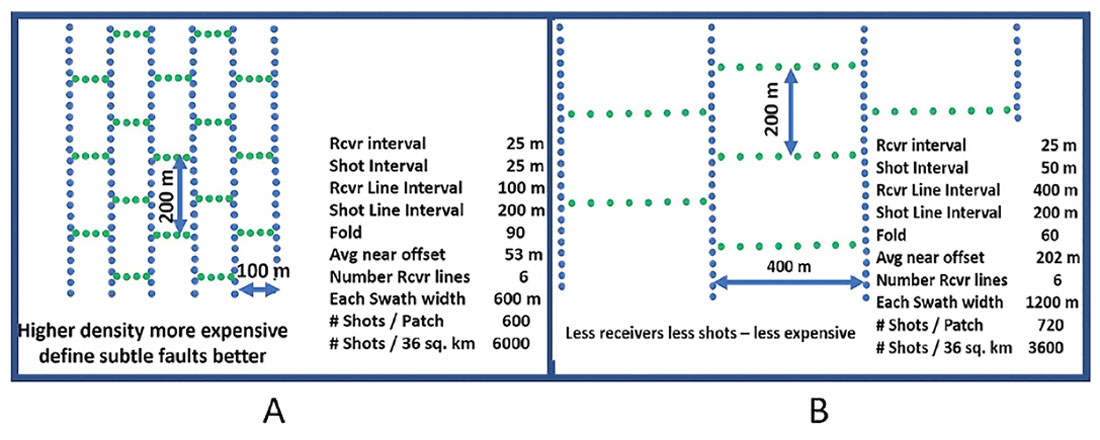
Also, the use of wireless telemetry has allowed for seismic “boxes” to record seismic data quickly and has resulted in the number of geophones on the ground being increased. It is important before seismic data is acquired that the survey parameters are chosen using survey design to understand the number of shots and receivers needed to optimally acquire data at the zone of interest.

The benefits of high density seismic data are finer spatial sampling, which reduces aliasing either steeply dipping reflection energy or noise (Lansley et al., 2007); and second, enhanced statistics which improves many processing steps such as deconvolution, statics, velocity evaluation, noise suppression, multiple attenuation, 5D Interpolation and migration (Lansley et al., 2007).

Depth Imaging

Depth Imaging handles velocity variations in the overburden between wells (Rauch-Davies, 2018). This allows the zone of interest to be better positioned in the seismic and thus reduces the risk of getting out of zone and “porpoising”. Staying in the zone of interest will also increase the production (Rauch-Davies, 2018).

Another issue is lateral velocity variations, which blur the imaging of fault planes and steep dips and which cause lateral mispositioning of key geological features (Rauch-Davies, 2018). Better resolution of subtle faults (Rauch-Davies, 2018) will help to reduce issues in the horizontal well such as fault planes that may act as thieves by diverting fluids and proppant to lower horizons or that may be the source of induced seismicity.

Depth imaging allows better horizontal well planning and reduces the uncertainty of fault avoidance (Young et al., 2009).

Better velocities that lead to better stacks

A byproduct from prestack depth digration is a better velocity field produced from the reflection tomography which utilizes a general ray-trace modeling-based approach (Bishop et al., 1985, Stork, 1992, Wang et al., 1995, Sayers et al., 2002; Satinder and Huffman, 2006) that improves the spatial resolution of the seismic velocity field (Sayers et al., 2002). Traditional picked velocities are spatially coarsely sampled and the short wavelength variation in the stacking velocity field is lost (Suaudeau et al., 2002). This leads to poor stacking in areas where there are strong lateral variations in the seismic velocities and blurring of subtle faults. AHDHRC velocities increase the resolution and bring out subtle faults within the seismic by providing flatter gathers. Reflection tomography produces a dense horizontal and vertical sampled velocity field (Satinder and Huffman, 2006) that can be used to produce a pore pressure volume.

The reflection tomographic velocity field can also be improved using automatic high density, high resolution, continuous (AHDHRC) residual velocities calculated using the T program, that is essentially a reverse radon program where parabolas from the radon are fit to the data to determine  that is utilized to correct the velocities; or, Swan’s (2001) Residual Velocity Indicator (RVI) that reduces the error within the gradient due to residual velocity (Spratt, 1987; Swan, 2001).

Overlaying tomographic or AHDHRC velocities over the seismic section illuminate the behaviour of the faults, such as whether it is leaky or a sealing fault (Kan and Swan, 2001) and it can bring out possible compartments within the geology that may affect production.

Frequency enhancement

One of the issues with seismic data is tuning. In seismic, a thin bed is less than one quarter of the wavelength and the wavelength is equal to the P-wave velocity or interval velocity divided by the dominant frequency. The higher the frequency, the better the vertical resolution. Therefore, some prefer to do time-variant whitening before they do inversion to enhance the resolution and attempt to remove tuning effects.

If there is tuning, the difference between the top and the bottom of the layer cannot be resolved. There are two prominent methodologies to accomplish whitening or spectral enhancement:

1. Time Variant Whitening involves passing the input data through many narrow bandpass filters and then determining the decay rates for each individual frequency band (Chopra, 2010). The inverse of these decay functions for each frequency band is applied, and the results are summed (Chopra, 2010). In this way, the amplitude spectrum for the output data is whitened in a time-variant way (Chopra, 2010);
2. Coloured inversion enhances the spectrum by matching the seismic data spectrum to the same spectral trend as the well logs in the area (Lancaster and Whitcombe, 2000). It shapes the inverted (Impedance or ρα) data spectrum to the geological impedance spectrum calculated from well data utilizing an operator. It is made without the use of a low frequency model and a wavelet. There can be errors in the wavelet estimation method of matching seismic to well reflectivity. The small errors in this single wavelet can manifest themselves as consistent errors in the inversion (Lancaster and Whitcombe, 2000).

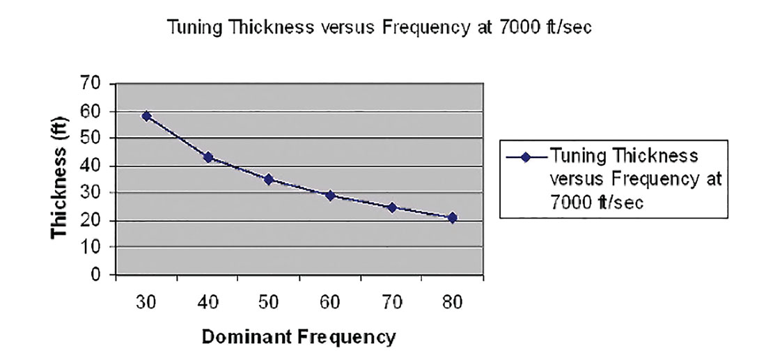
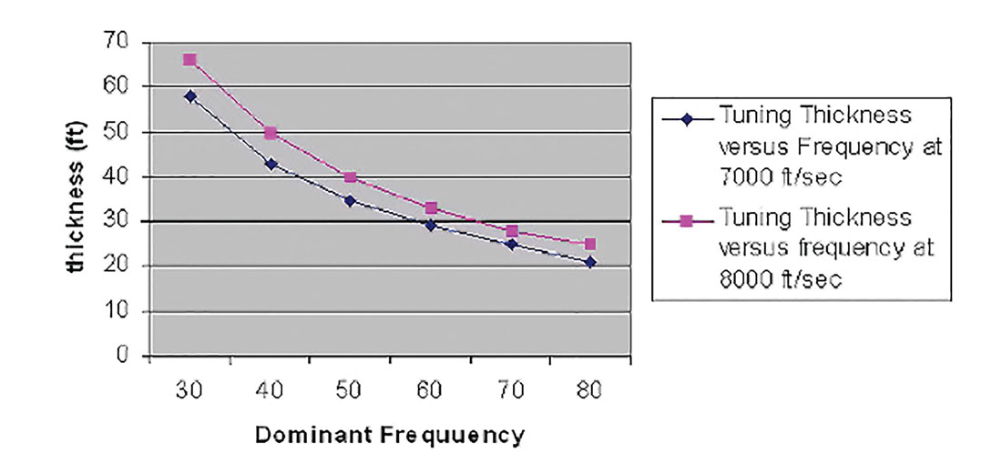
As can be seen in the chart above, the faster the rock, the less resolution, so with high impedance rocks such as carbonates, tuning may become an issue.

Acoustic Impedance

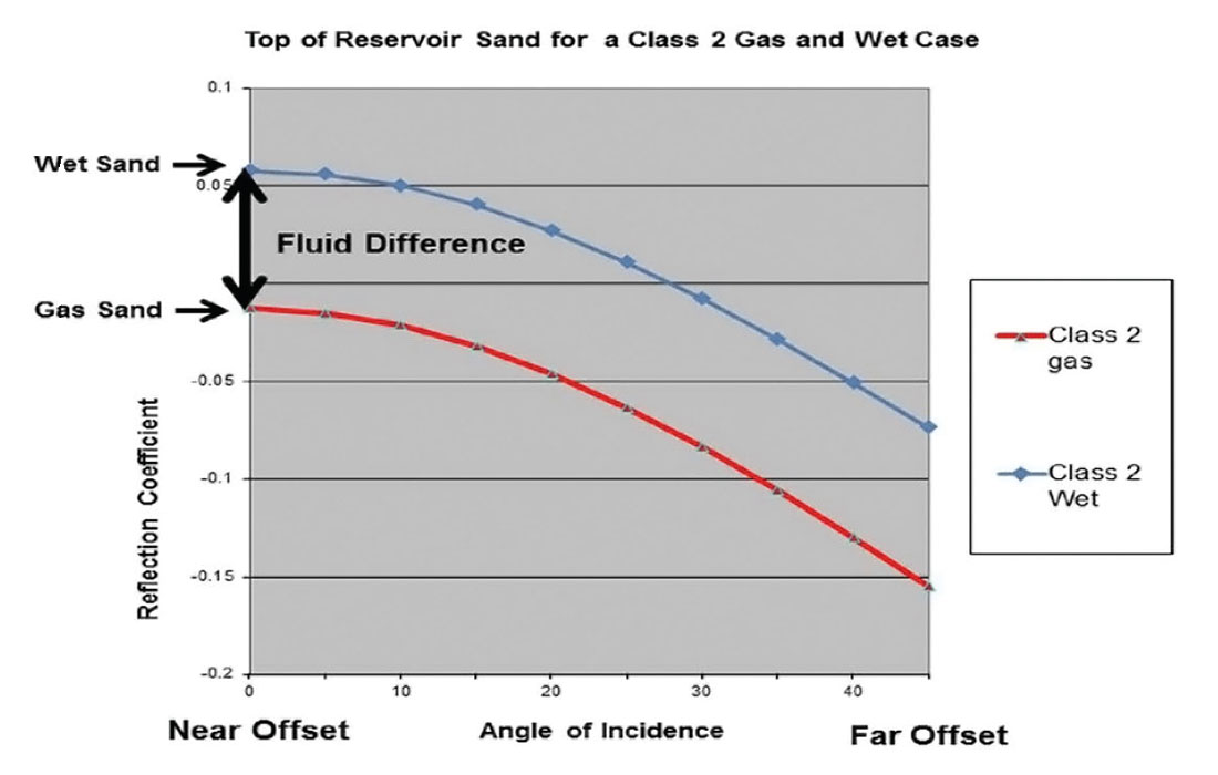
Acoustic Impedance is inversion of the near offset stack. With the near offset stack, the angle of incidence is low, so the energy is going straight down and coming straight up as it is reflected off the rock interfaces; therefore, the amplitude is equal to the reflection coefficient. The near offset stack tends to have higher frequencies and we have flatter gathers on the nears, which gives us a better stack.

The acoustic impedance is related to numerous rock properties such as:

1. Fluids – As shown in figure 5 the difference between fluids can be seen on the near offsets;
2. TOC – In the Montney, Sharma, Chopra and Ray (2014) showed that there was a strong linear correlation between the Passey et al. (1990) methodology for detecting organic-rich depth intervals in shale zones and AI;
3. Porosity – There tends to be a linear relationship between porosity and AI.

This linear relationship makes sense if, as shown in figure 5, it is related to fluids, because porosity is really where the fluids are stored in the rock.

The Coloured Inversion of the near offset stack produces a relative acoustic impedance.

To acquire near offsets in a swath 3D survey, the receiver lines need to be tightly spaced which increases the density of the survey and increases the cost of the survey. The value of acquiring the near offsets to image subtle faults that may affect the fracking of the well does offset the increase in cost to acquire a high density seismic survey.

The far offsets are easier to acquire and do not affect the overall cost as much.

Structural Smoothing

Structural Smoothing will remove noise, but it will preserve relevant details such as structural and stratigraphic discontinuities. Enhancing structural and stratigraphic discontinuities in a Coloured Inverted Acoustic Impedance can reveal subtle faults within the seismic data. Inputting this volume into structural attributes such as chaos, curvature, and semblance analysis can reveal subtle faults not seen in the seismic data.

Conclusion

The ability to see subtle faults within the seismic data while planning the horizontal wells can lead to changes in the completions, which can reduce induced seismicity, lower costs during fracking and increase production by allowing the horizontal well to stay in zone longer. This is like doing a pore pressure analysis for a Deepwater well to minimize issues caused by intersecting an unknown high pore pressure zone, which may cause a blowout like the Alpha Piper.

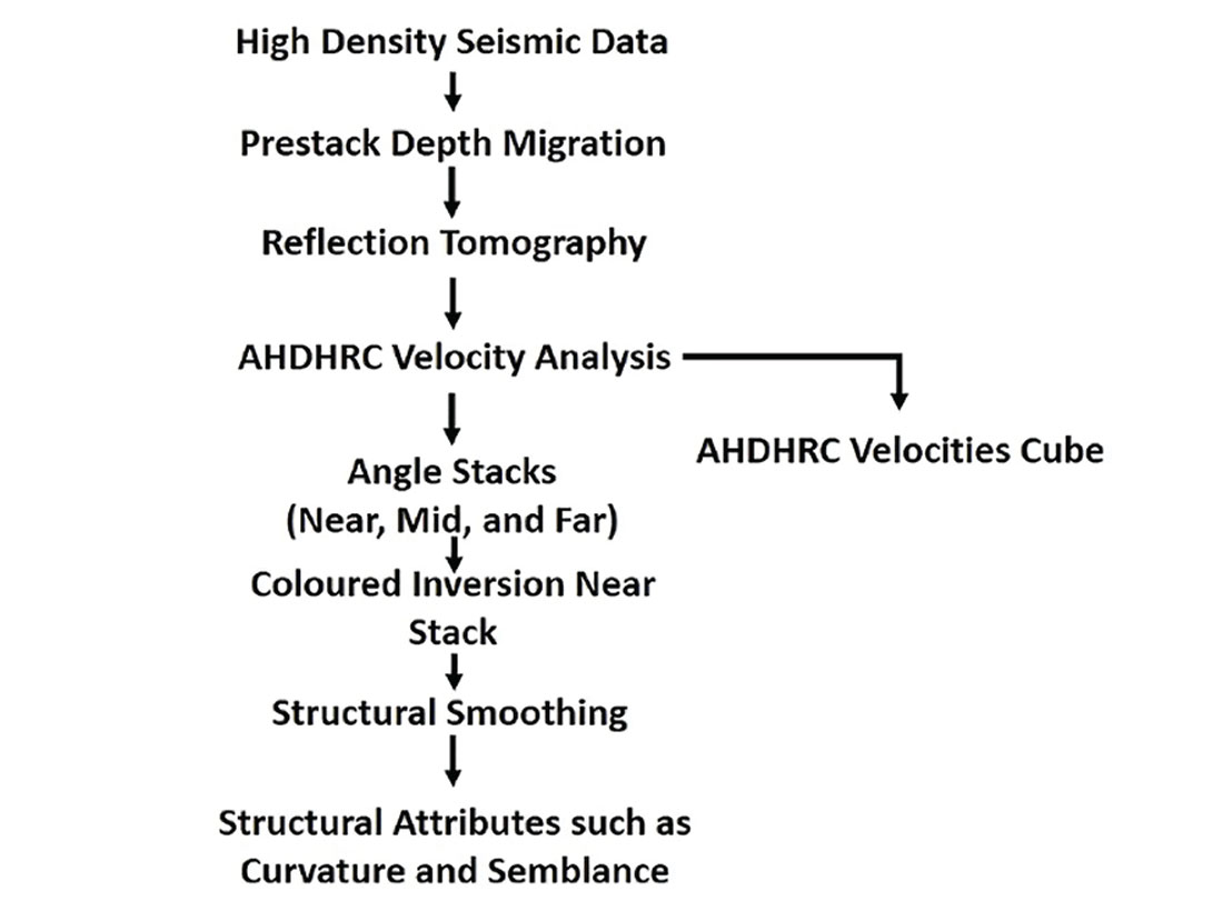
The ultimate seismic processing flow to enhance subtle faults is shown in Figure 7.