Filling in the Gaps in Our Understanding of Converted-Wave Fold

The “Problem”

For a newcomer to converted-wave processing, one of the most confounding things that is encountered early on is the realization that the fold of P-S data can differ so much from the fold of ordinary P-P data. For example, Figure 1 shows the PP and P-S fold distributions for an actual 3-C/2-D line. The PS fold (sometimes called CCP fold, for common-conversion point) was calculated with a typical value of Vp/Vs = 2.0. For this line, a single receiver spread was laid out, and shots were fired from one end of the line to the other at each receiver station. There is a steady increase in P-P fold towards the middle of the line, as expected, but the P-S fold oscillates from bin to bin by about a factor of two. These oscillations are obviously undesirable since they would produce oscillations in the signal-to-noise ratio.

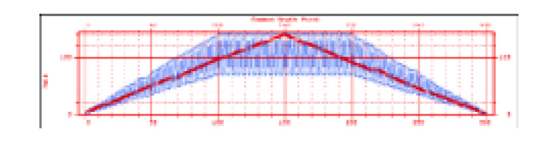
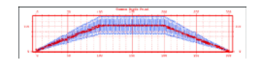
The main purpose of this article is to explain that the fold differences between P-P and P-S data depicted in Figure 1 are more apparent than real. The rapid oscillations are due to the fact that we are not calculating fold accurately: the illumination of the subsurface is actually uniform. Once fold is calculated more accurately (in a way that represents subsurface illumination), the P-S fold becomes much more uniform. Figure 2 shows the P-S fold calculated in a more accurate fashion (in red) for the same geometry as for Figure 1. So P-S fold and P-P fold are not so different after all.

It is not quite this simple, however. The way we normally calculate it, fold indicates the number of stacked traces within a bin. So it is not just the way we calculate fold that needs to be changed to be more accurate, the way we calculate stack needs to be more accurate as well.

When it comes to understanding the differences between P-P and P-S fold, newcomers have no reason to feel badly for being confused. This aspect of converted-wave processing has led to much confusion through the years. The most common solution to the “problem” is to alter the distribution of shots and receivers on the surface so the fold (when calculated the ordinary way) is uniform for both P-P and P-S surveys. The trouble is that this can lead to unnecessary expense and complication. It is better to understand the real source of the problem, and only make acquisition design changes if they are absolutely necessary.

How Should Fold be Calculated?

What a simple question! What could be easier than calculating fold? We add up the number of traces within each CMP bin, and that is the fold. At least that is the way fold has been calculated since the beginning of CMP processing.

However, notice that this simple method does not take into account whether the midpoints lie in the middle of the CMP bin, or are scattered about the bin. This simple method corresponds to the way in which we calculate a stacked trace—we add together all the traces that fall within a CMP bin regardless of whether the midpoints occur at the centre of the bin or not. This is known as nearest-neighbour interpolation. As you would suspect, there is a small amount of smearing of the signal that occurs when the midpoints do not occur exactly at the bin centre.

If we want to take into account the actual location of the traces within each CMP bin during the stacking process, some sort of interpolation is required. But what type of interpolation is appropriate? In order to know what type of interpolation is appropriate, we need to understand the nature of the signal we are dealing with.

Bandlimited Rays

A plot that shows the scatter of midpoints for a seismic survey indicates the positions are halfway between the source and receiver positions for each trace that has been recorded. Each midpoint on this type of map is meant to indicate the exact location at which a ray from a source reflects from a flatlying subsurface reflector and returns to a receiver. So it shows all the points are illuminated on the subsurface reflector.

However, it is unrealistic to consider a seismic ray as reflecting from a single point in the subsurface. It is important to remember that rays are fictional constructs we use for aiding our understanding of how waves propagate in the subsurface. Since we are dealing with spatially bandlimited seismic wavefields, it is appropriate to consider rays as having an effective width that gets more narrow as the bandlimits of the wavefield increase. So “fat” rays would not be able to resolve features in the subsurface as well as “thin” rays.

If we assign to each reflection point a finite width that is related to the spatial bandlimits of the wavefield, then we can expect fold maps to become more uniform when there is considerable midpoint scatter within bins. This is essentially the technique that was used to generate the smooth fold plots in Fig. 2 when the standard method produced the irregular fold plot in Fig. 1. The question is, however, what form of interpolator is able to to represent bandlimited rays, and what effective width of the rays should be used?

Binwidths and Bandlimits

When we choose the bin size for a seismic survey, we are actually making an assumption about the highest wavenumber that we believe could be present in the data, and preserved in processing. The chosen bin width is the spatial sample interval that is required to preserve the highest (Nyquist) wavenumber assumed will be present in the final image. Just choosing a particular bin size does not mean that all wavenumbers up to the assumed highest wavenumber will actually exist. It simply means that, if wavenumbers up to that particular Nyquist wavenumber exist in the signal that comes back to the surface, then processing the data with that bin size should be able to preserve those highest wavenumbers.

A sinc function, shown in Fig. 3, is the Fourier transform of a boxcar function. Because of Shannon’s sampling theorem, we know that a sinc function is capable of preserving all wavenumbers up to the assumed Nyquist bandwidth. Therefore, this sinc interpolation is the ideal type of interpolation for our purpose. In theory, at least, a sinc function is the “mildest” possible interpolator we could use, it makes no additional assumptions about the data beyond what has already been made in choosing the bin size.

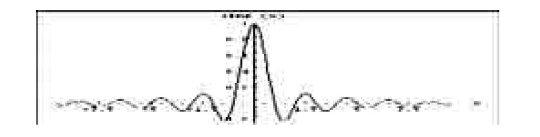
A sinc function may seem like an unusual function to use for interpolation for two reasons. First, it is infinite in length (any implementation must use a finite approximation to this function.) Second, it has negative as well as positive values. This means interpolating a trace will often involve multiplying that trace by a negative number before adding it to the stack. This method does yield the desired result once all calculations are complete, even though it may not be obvious it should. Other commonly used interpolators, such as linear or Gaussian interpolators, on the other hand, use only positive multipliers. These interpolators can give similar results to the sinc interpolator at low wavenumbers, but will attenuate high wavenumbers if they are present.

To preserve all wavenumbers up to the assumed Nyquist wavenumber, the distance between zero crossings of the interpolating sinc function is equal to the CMP bin width, except for the main lobe, where the separation is two CMP bin widths. To interpolate a trace with the sinc function, the centre of the function is placed at the trace’s midpoint, and the trace is multiplied by the value of the sinc function at each bin centre and the result is added to the stack. This amounts to a convolution of the trace with the sinc function. The final stack is normalized by the sum of the sinc function multipliers at each bin centre. Notice that if a trace’s midpoint is at a bin centre, this operation will multiply the trace by 1 (the central value of the sinc function), add it to that bin, and add zeros to all other bins.

Sinc-function spatial interpolators are commonly used in wave equation processes such as DMO and migration, and we are simply using the same assumption in the simple process of stack. By doing so, midpoint scatter within each bin is properly taken into account during stack and fold calculations.

A 3-D Example

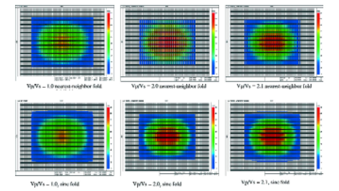
The type of interpolation that is used in fold calculations can be very important when designing 3C/3D surveys. For example, Fig. 3 shows how misleading nearest-neighbor fold calculations can be in the design of 3-D, 4-C OBC surveys with orthogonal shot and receiver lines. In this example, the source and receiver intervals are 50m, the source line separation is 100m, and the receiver line separation is 300m. The nearest neighbor fold calculation for Vp/Vs = 2.0 indicates that the fold periodically drops to zero along many lines, whereas sinc-function interpolation indicates that the illumination of the subsurface is actually smooth, without gaps in the fold. Notice as well that a small increase in the assumed Vp/Vs from 2.0 to 2.1 produces a big change in the fold map with nearest-neighbor interpolation, but not with sinc interpolation. Finally, notice that the CDP fold calculation (Vp/Vs = 1.0) is also smoother and more accurate with sinc interpolation.

Discussion

Many of the algorithms in the initial processing of P-S data, such as velocity analysis and statics, require that prestack traces be gathered into CCP bins, but not interpolated. Since these algorithms do not require highly accurate positioning of the data, the simplest approach for avoiding the problems with fold variations from bin to bin is to use a value of Vp/Vs that yields a fairly uniform fold. More accurate interpolation, with the correct Vp/Vs, only needs to be performed later in the processing.

One way of understanding the calculation of fold is in terms of “fat” operators. We are proposing the use of a “fat stack” operator which takes into account the bandlimited nature of the seismic data, and overcomes spatial sampling problems.