Five-dimensional interpolation: New directions and challenges

Five-dimensional (5D) interpolation has been in the industry for almost ten years now, and has become widely accepted and used. There are now a variety of implementations, with different algorithms and flavors. Our understanding of interpolation has grown greatly in the last decade because of its use in increasingly challenging scenarios. A few years ago interpolation was targeted to remove sampling artifacts in the stacked image from prestack migration; today it is used to improve amplitude analysis in common image gathers and time-lapse studies, which are much more demanding. However, answers for many of the questions that this technology created at its beginning remain unclear, and differ among experts. Here I discuss some of these questions in the context of land surveys and point to directions where interpolation may be heading.

Introduction

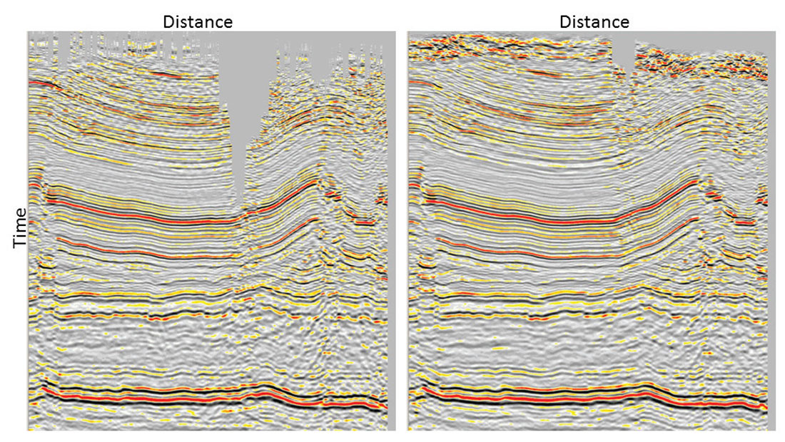
Multidimensional sampling is not easy to visualize or understand, because different dimensions are linked through physics in complex ways. Often the sampling problem is wrongly considered as if frequencies and wavenumbers along each dimension were free to take any value up to Nyquist. In reality, seismic frequencies can only take a limited bandwidth along each dimension and are connected across dimensions through the wavefront curvatures in the five-dimensional seismic volume (e.g. inline, crossline, offset, azimuth, frequency). Although it is not easy to exploit this knowledge about the physics of the wave propagation, we can use it to constrain the data spectra to predict new traces. For example, we use band limitation and smoothness in the spectrum, and assume that data changes slowly as a function of frequency and wavenumber. In spite of only using approximations, interpolation algorithms have been highly successful by using spectral models from recorded traces to predict unrecorded data. The mechanism behind interpolation is to first remove from these models (spectra) artifacts produced by poor sampling, such as aliasing and noise, and then to invert them to predict the seismic data at arbitrary locations. This is possible since seismic data are redundant, for example because of overlapping of Fresnel volumes, and additional predicted traces do not need to be perfect to help migration algorithms. Although traces created from data interpolation contain only a portion of the information that a real acquired seismic trace would have, this is usually all a migration algorithm will keep after moving and stacking millions of samples. Figure 1 shows a prestack migration result with and without 5D interpolation. The migration result has clearly improved with interpolation even when the added data do not agree exactly with the unrecorded samples.

After almost ten years of application in the industry, some of the original questions about interpolation generate different answers or remain unclear:

1. What is the best output geometry design?
2. Which algorithms are more appropriate?
3. How does aliasing affect 5D interpolation?
4. Can 5D interpolation preserve diffractions (i.e fractures), AVO and AVAz?
5. How can we mitigate the effect of noise on interpolation?
6. What is next?

Output Geometries

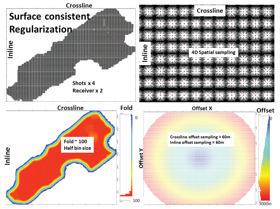
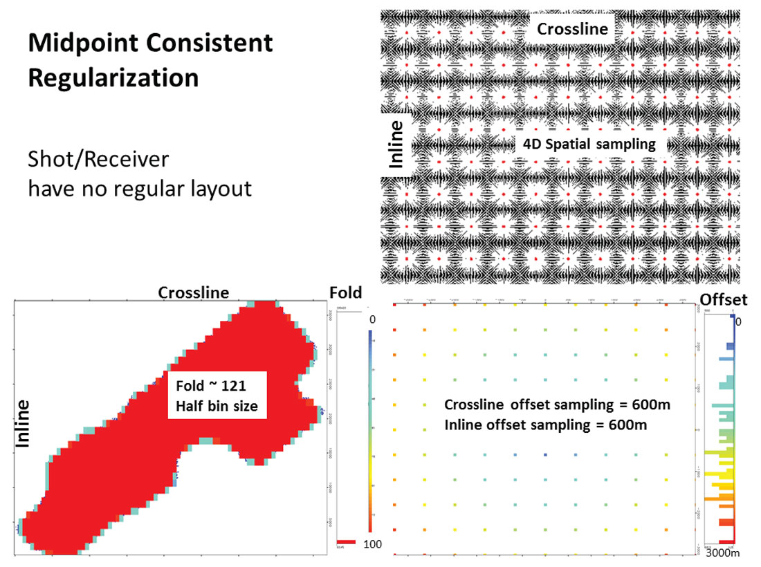
There are two trends when designing geometries for interpolation (Trad, 2009): (1) Acquisition-guided, or surface-consistent, geometries are obtained by creating new shots and receivers and letting midpoints, offsets and azimuths fall where they must (Figure 2), or (2) midpoint-guided, creating for every CMP a regular distribution in offset-azimuth or inline-crossline offsets (Figure 3). What is the difference? From the point of view of the algorithm there are few differences. However, some practical issues make the handling of the interpolated data different.

1. Surface-consistent data: keeping the output geometry similar to the input geometry permits a clear comparison between new and interpolated traces and, most important, new traces are close to where they were originally acquired. These geometries permit working on shot/receiver gathers which is important for most migrations except Kirchhoff and Gaussian Beam. Since the industry is moving to reverse time migration (RTM), this may become important in the future.
2. Midpoint-consistent data: On the positive side, each CMP has the same offsets/azimuths, which creates perfect common-offset vectors. This favors Kirchhoff and beam migrations – the strongest argument to follow this pattern. Also some studies such as multicomponent shear wave splitting or Amplitude Versus Azimuth (AVAz) analysis benefit from having a regular azimuth distribution. On the negative side, this design produces coarse offset/azimuth (or inline-crossline offset) sampling.

Additionally, for surface-consistent geometries, there are two alternatives: regularization, meaning perfectly regular shot/receiver layouts and disregarding original traces, or interpolation, meaning keeping original traces and adding more shots/receivers. Which is better? Again, there is no difference for the algorithms but there are some practical differences for processing flows. Regularization tends to produce better migration results and some algorithms do require data sampled on regular grids. Interpolation permits better quality control and a smoother transition between original and interpolated traces. For example, interpolated traces with poor quality can be discarded according to some quality flag, which can be fine-tuned by testing after interpolation.

Algorithms

5D interpolation requires algorithms that can manipulate large number of traces simultaneously. The first algorithm used in 5D was Minimum Weighted Norm Interpolation (MWNI) (Liu and Sacchi, 2004, Trad, 2009). MWNI is still one of the most popular algorithms because of its efficiency and amplitude preservation. These features come as a consequence of using regular grids after four-dimensional (4D) binning, which permits the use of Fast Fourier Transforms (FFTs). This enables the algorithm to infill large holes, since it can handle large data volumes simultaneously. Because the transformation from data to model (spectra) is performed by an operator with close to orthogonal properties (Trad, 2009), it achieves an almost perfect fit to the input data in very few iterations, which leads to excellent amplitude preservation. By contrast, algorithms that use discrete Fourier transforms on irregular grids instead of FFTs have operators that are more difficult to invert; in addition, they require weighting to compensate for irregular sampling, which has the potential to affect AVO and AVAz, in particular for land data with a highly variable spatial density.

However, matching irregularly sampled recorded data to regular grids brings many complications for MWNI, in particular for limited azimuth aperture surveys. For that reason, in marine processing it is more common to use algorithms which do not require 4D binning. Probably the more popular of these is Anti-Leakage Fourier Transform (ALFT) reconstruction (Xu et al, 2005, Poole, 2010). Although prohibitively expensive in 5D until recently, it is now often used because of its ability to deal with aliasing and strong noise, and most of all its flexibility. ALFT differs from MWNI in two respects: first, ALFT uses exact recorded locations (although MWNI can also be implemented at exact locations); second, ALFT uses an efficient ad-hoc procedure to solve for one wavenumber at a time, which increases flexibility for noise attenuation. MWNI uses instead a conjugate gradient solver to solve at each frequency all wavenumbers simultaneously, which makes it excellent for amplitude preservation.

Other algorithms based on regular grids used for 5D interpolation in the industry are Projection Onto Convex Sets (POCS) (Abma and Kabir, 2006), and rank reduction of Hankel tensors (Trickett, 2013). Similar to MWNI, these methods suffer an increase in the number of equations to solve as they attempt to reduce binning errors. This is compensated by the use of fast algorithms, and large windows, which give more data to interpolate from. There is a complicated trade-off between window sizes and binning errors but usually regular grids work well on land wide-azimuth geometries such as orthogonal ones, but not on marine narrow-azimuth streamer acquisitions. Recently hybrid approaches have been implemented which apply regular grids with an additional interpolation to minimize binning error which helps for far offsets (Jin, 2010, Li et al, 2012, Wang and Wang, 2013).

Aliasing

Historically, interpolation has been thought of as the problem of unwrapping aliasing since simple sinc interpolation (adding wavenumber components with zero values beyond the original Nyquist frequency) is sufficient to interpolate non-aliased data. However, the meaning of aliasing is unclear for prestack five-dimensional data because sampling is always irregular along one or more of the five dimensions. Furthermore, a signal that appears aliased in one dimension may not be aliased in another and aliased frequencies in multi-dimensions may not overlap in the multidimensional spectra, so it is usually possible to separate them by applying constraints. As a consequence, 5D algorithms can get around aliasing more easily than lower dimensional interpolators by filtering lower temporal frequencies and carrying information about the localization of wavenumbers to higher temporal frequencies.

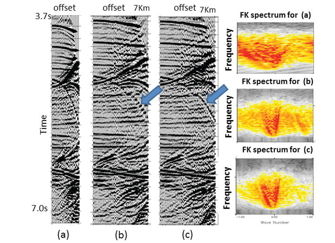
The situation becomes more difficult when all spatial samples are located on regular grids and aliasing occurs in all directions simultaneously. This never happens in five dimensions, but it may occur on narrow-azimuth marine streamer data. Typical solutions in such cases are to apply a spectral mask, not only at the first temporal frequency, but also at higher frequencies. Figure 4 shows a synthetic case from a complex salt environment, which is more difficult than most real scenarios because it has regular sampling and aliasing in all dimensions. In this case the use of standard band limitation plus an artificial sampling perturbation to the interpolation grid helped to interpolate beyond aliasing. In practice, all land surveys have irregularity at least along offsets and azimuths, and therefore are much easier to interpolate than this example.

Amplitudes, fractures, diffraction preservation

Most 5D interpolation techniques use similar assumptions: sparseness of plane wave events (small windows of data contain few wavenumbers). Since this assumption is not realistic, the success of interpolation lies in defining windows with appropriate parameters (overlap and size) to approximate the sparse wavenumber assumption. In 5D interpolation, each window typically contains thousands of common midpoints, hundreds of offset bins, and several dozens of azimuths. If these windows are too small, there are not enough traces to interpolate from. If the windows are too big, interpolation may not converge either because events become too complicated and break the sparseness assumption, or because the optimization problem becomes too large for the algorithm to converge in reasonable time.

Algorithms that use regular grids are usually good at preserving all complex features in the data, but they are affected by binning and window problems. Conversely, algorithms that use exact locations do not have binning issues, but they may suffer from slow and insufficient convergence. Algorithms that use regular grids have a limitation on the percentage of live traces versus the number of empty bins on the grid. For example, MWNI can infill a regular grid even if the number of live cells is as low as 3%, which is probably as sparse as can be done realistically with most algorithms. Windows that lie on the borders of surveys or on gaps, at shallow times or far offsets, usually have less than this percentage and often exhibit problems. Overlapping windows both help with these issues and filter out unrealistic information created during interpolation. In a typical half-overlap, each trace is created four times using four different subsets of the input data. When these four versions of the same trace are combined together (e.g. using a weighted stack), only consistent features stack up. When information is insufficient to constrain the high frequencies, for example inside large gaps, high frequencies tend to be attenuated during the process of stacking overlapping traces.

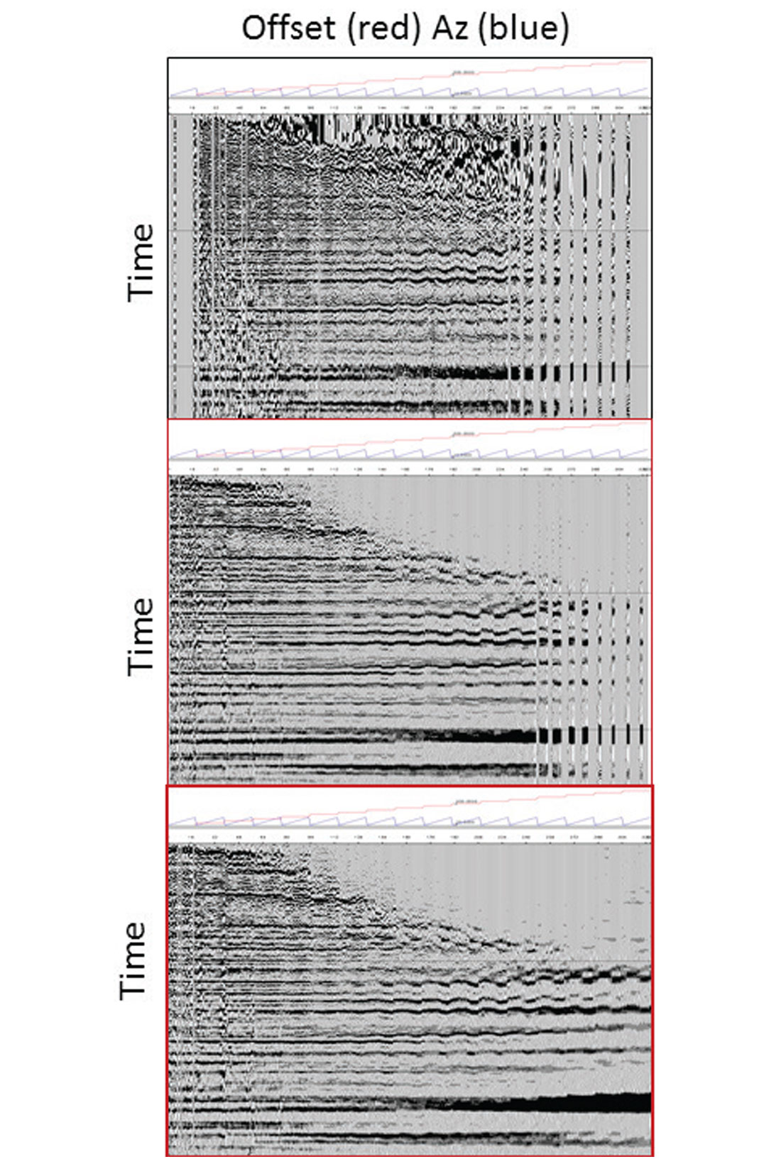
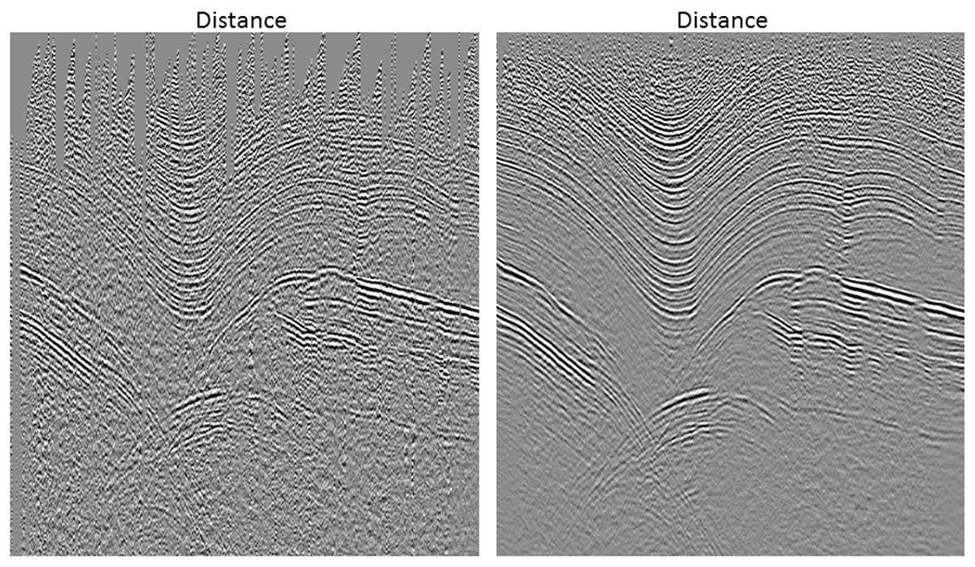
Optimal 4D binning of irregular data can become difficult because the midpoint-offset-azimuth distributions are variable across the survey and across the offsets. To properly handle binning requires taking into account data sampling independently from window to window. Using coarse intervals destroys coherence unless data are flat. Diffractions are particularly susceptible to this problem, and tend to be the first feature of the data to be affected by coarse binning. Long-offset data are also susceptible to binning problems because of residual moveout and AVAz. Figure 5 shows a CMP gather indexed by offset and azimuth (top). In the middle of the figure we see the same gather after interpolation with a fixed regular azimuth binning that shows problems on the Horizontally Transverse Isotropy (HTI) signature at long offsets. By applying the same interpolator with adaptive azimuth binning we obtain an interpolated gather with proper HTI signature (bottom). In this binning approach, each interpolated window uses its own binning parameters calculated automatically to adapt to variable sampling across the survey. This adaptive binning is also crucial to properly preserve diffractions in complex structures. Figure 6 shows a limited-azimuth stack on a complex area before and after interpolation.

Diffractions have been properly preserved but they would have been attenuated if binning had been too coarse.

Noise and Interpolation Strategies

Interpolation acts as a random noise attenuator because it can only predict coherent energy, but there are already many processing tools to tackle random noise. Coherent noise, on the other hand, can barely be distinguished from amplitude variations and data complexity unless strong assumptions are imposed. An interpolator designed to attenuate coherent noise could fail to preserve amplitudes on poorly sampled complex data. Only by introducing additional information and strong assumptions about the data can the algorithm be made robust to noise. One type of additional information most interpolations use are velocities. Applying normal moveout to the data before interpolation simplifies the task by reducing the wavenumber bandwidth (and aliasing) in the offset direction and reducing binning error if a regular grid is used.

Another way to supply information that helps to reduce noise is to incorporate a guide. An example of such a method is Double Guided Interpolation (Trad and Clement, 2012) (Figure 7). At each frequency, the algorithm processes the main data set and a secondary (guide) data set which has been heavily filtered by strong noise attenuation. The guide data set is interpolated first and then the differences between the interpolated guide and the main data (residuals) are interpolated and added into the first interpolation. The interpolation of the residuals requires few iterations since it needs to adjust only small variations. The process can be applied to clean a data set without interpolation, or to interpolate a noisy data set. This method is useful as long as a proper guide can be obtained. The process can be considered from three points of view: a) restoring signal lost during processing, b) interpolating a noisy data set using additional information provided by a secondary data set or c) adjusting the phase of the data first (guide) and then the amplitudes (recorded data). Several combinations are possible, but usually spectral information taken from the secondary data is used to guide the interpolation of the main data.

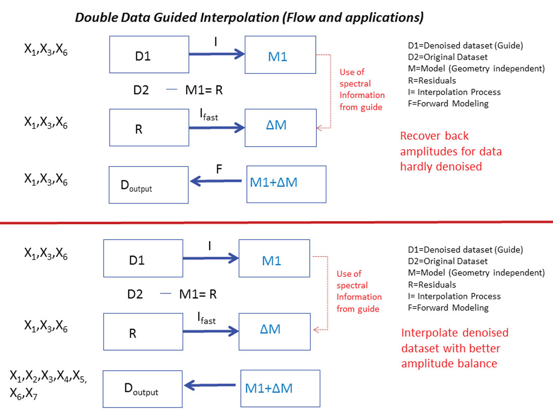
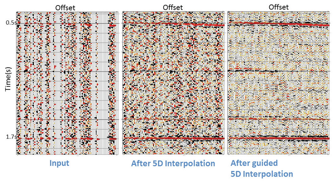
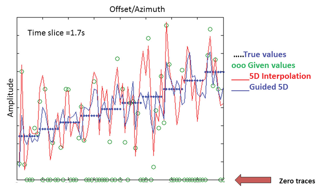
Figure 8 shows a synthetic example with four reflectors and clearly defined AVO trends. For clarity, only the last reflector AVO signature is shown on Figure 9. Green points correspond to existing traces and blue dots represent the actual amplitude trend used to create the data before adding noise. Standard interpolation without a guide increases the data density by four times to produce the data in the middle of Figure 8. The trend is well preserved, although we see strong variations in amplitudes produced by the leakage of the noise into the model. By incorporating a guide containing the reflectors at the correct positions but with wrong amplitudes, interpolated amplitudes follow the correct trend more closely (Figure 8 to the right, blue line in Figure 9).

Other challenges and directions

5D interpolation makes assumptions that break down in some scenarios. Normally 5D interpolation uses midpoint as two of the four spatial coordinates because these two dimensions are dense and well-populated. A problem occurs on multicomponent data, where the asymmetry of the converted wave ray path leads to time-variant midpoints. Accommodating variable midpoints in the time domain brings many operational difficulties, since most algorithms work on temporal frequencies. Midpoints also change with time in ocean bottom surveys (OBS). Interpolation in both scenarios is possible by using an asymptotic common reflection midpoint. This assumption is, however, poor for shallow data and insufficient in the case of OBS with PS data, where the effects of both different P and S propagation and different shot/receiver elevations accumulate. This is a serious issue as both types of data benefit from interpolation, since land surveys are usually designed for PP data not PS, and ocean bottom nodes are typically located at coarse intervals. A possible solution is to abandon the concept of midpoint for this type of surveys and work instead on survey coordinates (shot and receiver coordinates). The difficulty with this approach is that these coordinates are usually coarse and aliasing becomes a problem. Another scenario where interpolation breaks down is when the signal is below the noise level and only more complex operators with additional physical information can recover the signal.

A possible improvement on 5D Fourier-type interpolation is decomposing the data in physical wavefields which capture the geophysical information obtained through processing and velocity analysis. In this respect, an obvious candidate to replace interpolation is Least Squares Migration (LSM). LSM was first proposed fifteen years ago (Nemeth et al. 1999), but has been held back by the success of interpolation, which is simpler and more efficient. Also, LSM is difficult to implement correctly because it is sensitive to amplitude errors during processing and to approximations in the migration operator. In practice, fitting input amplitudes by itself does not lead to a better image, and complex additional constraints are required to achieve attenuation of the sampling artifacts, something that interpolation achieves with less effort. However, a proper LSM in acquisition coordinates has the potential to deal with many of the situations where 5D interpolation breaks down. There have been some novel approaches to make LSM more robust to the amplitude problem. One approach that fits in the context of this article is to use the migration operator as an interpolator. In this approach unrecorded shots and receivers can be predicted from migrated common image gathers by using the modeling operator. These traces are accumulated during iterations and included in later iterations in a similar way to POCS interpolation, allowing a relaxation of the migration antialiasing filter as iterations progress.

Summary

5D interpolation has become a mature technique in the last decade because of its extensive use for wide-azimuth surveys. There are, however, many unsolved issues and a large effort has been made worldwide to develop new algorithms. A general trend has been to reduce issues related to binning by using algorithms that can handle exact coordinates. These methods require special care in the use of weights to handle amplitude preservation but they are becoming easier to use and more flexible. In other cases, the problem has been approached by hybrid techniques where the irregularity is dealt with an additional bin centering during the mapping to the regular grid. Another trend is to use more information by handling two versions of the data either for noise attenuation or for multicomponent data. Developments of techniques that work in acquisition coordinates instead of midpoint coordinates have become necessary to handle OBS and PS-converted waves. One such technique is least-squares migration, which represents another trend: the use of basis functions that can capture geological information. Although more computer resources are required, the processing flow simplifies because the sampling issues are dealt with directly where they cause the problem, inside migration. This permits one to use all geophysical information inside the computation kernel and work directly from topography.

Acknowledgements

The author would like to acknowledge to Sylvestre Charles from Suncor, Nexen, CGG US Data Library, Carlyn Klemm, Candy Krebs, Rodney Johnston, Jesse Buckner, Peter Lanzarone from BP North America Gas Resource for providing show rights. My thanks to several CGG colleagues and clients that provided the real data examples and insight through discussions across a decade of 5D interpolation. Special thanks to Sam Gray for his help and discussions on this paper.