Fourier Domain Regularization 5D and More

Summary

Global multi dimensional regularization has become a widely used tool in seismic data processing. Many advantages of regularization in the Fourier domain come with some serious problems. In this paper we consider the intrinsic properties of the Fourier transform to identify problems and limitations of the method.

A practical and efficient iterative multi dimensional regularization technique is proposed to overcome the strategic pitfalls of the Fourier transform. The results of application on different 2D and 3D data sets are discussed.

Finally, we show how the same multi dimensional Fourier regularization technique can be used as a random and coherent noise suppressor.

Introduction

There are plenty of reasons to perform regularization, such as to increase spatial sampling, create a regular grid, reduce noise, and improve prestack imaging and AVO analysis.

Converting seismic data into the frequency wave number or multi dimensional wave number domain is a natural tool for data regularization. However, its efficiency comes with some serious problems usually characterized as "spectral leakage". A clear understanding of what causes such phenomena will help us to develop an improved tool to perform interpolation, multi dimensional regularization, noise suppression; as well as any other operation in the frequency or frequency wave number domain in a meaningful way.

Method

To perform regularization of prestack seismic data, we create a new desired regular grid filled with the available input data, positioned at the nearest grid node, and with zero data at all other locations. Gridded data are first converted into the frequency domain and then into the multi dimensional wave number domain.

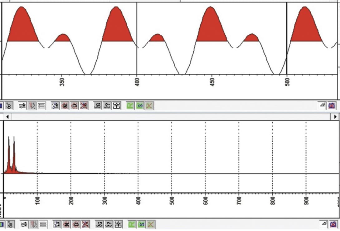
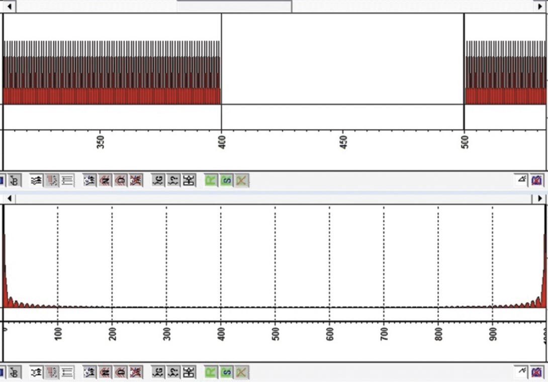
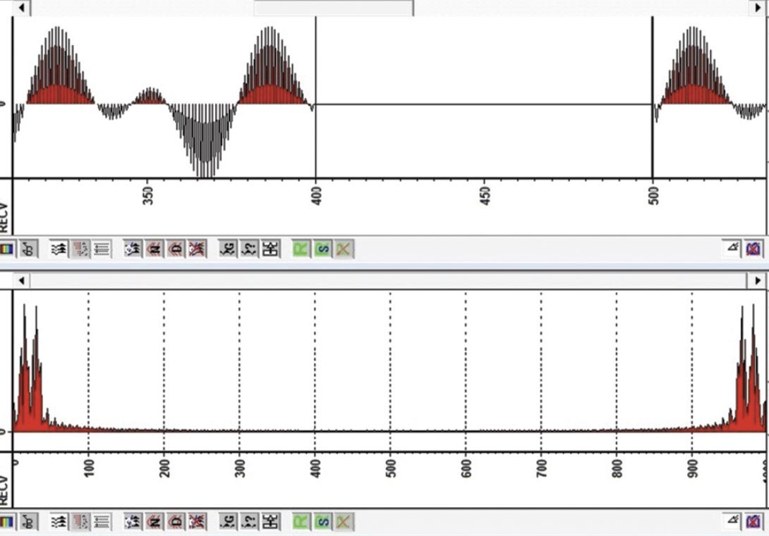
All zero traces can be considered to be a result of multiplication of the full wavefield by the sampling operator. Therefore, this final spectrum is the result of the convolution of the full data spectrum with the Fourier transform of the sampling operator. Figure 1 shows spectrum distortion of a signal consisting of two sine waves caused by both a gap and upsampling. Two main problems arise: spectrum “repetition”, caused by the upsampling operator, and amplitude distortion, caused by the gap. We have to keep in mind that there is always some amplitude distortion caused by zero padding in time and space. This spectrum distortion is also known as “spectral leakage”; which means that each original spectrum component affects others and components with stronger amplitudes have more impact, especially on the nearest components.

These problems should be dealt with during (and simultaneously with) the regularization process.

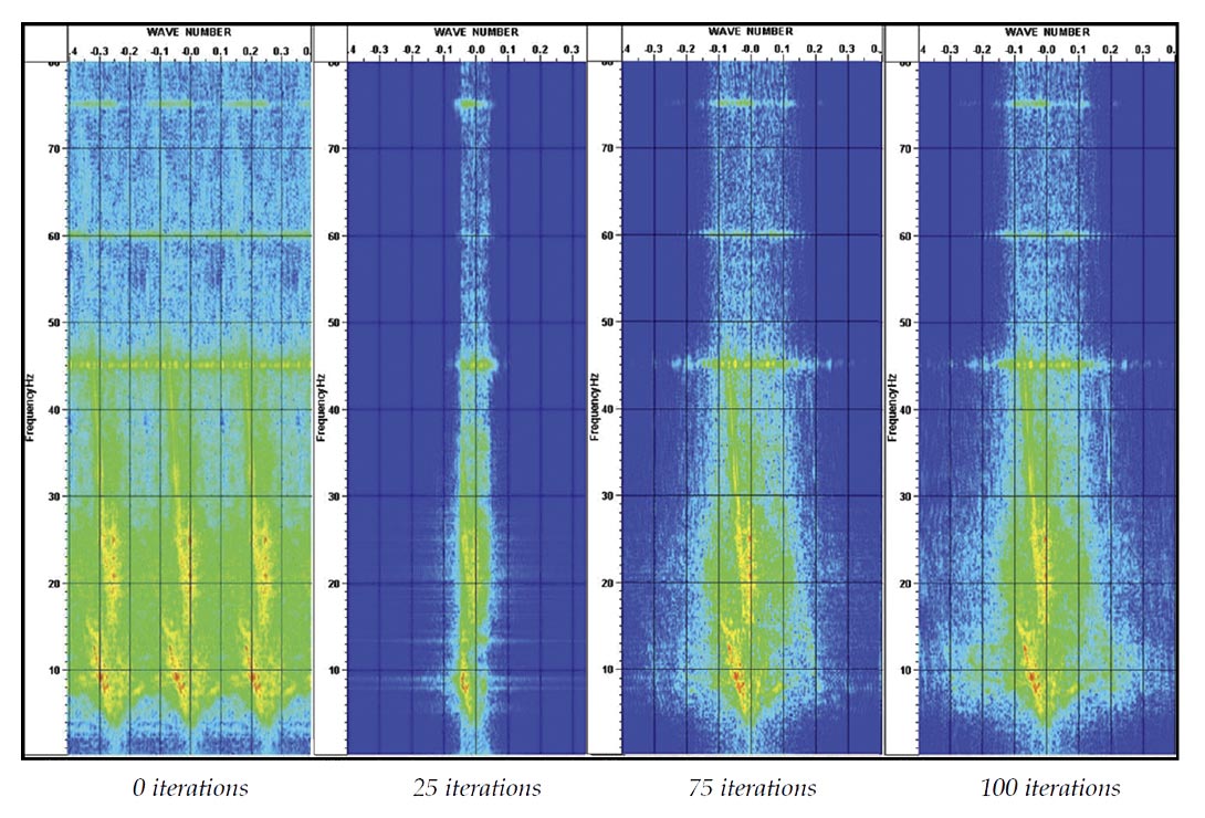
To overcome these problems, we adopt the following procedure. At each iteration, only those spectrum components, bigger than a specified threshold and within current wave number limits, are selected and accumulated in the output spectrum. After the inverse wave number Fourier transform, the resulting grid of traces is first reduced to only the original trace positions. Those “original position” traces are then subtracted from the input. Thus, by subtracting the strongest components, we reduce the strongest distortion of weaker components. The result of the subtraction will then be forward transformed, ready for the next iteration. The threshold is reduced at each step of the procedure. To prevent data aliasing, especially if substantial upsampling is the objective, the search area of the spectrum is truncated at the current values of the maximum wave numbers in all directions. Thus, the iterations first concentrate on high amplitude data near small wave numbers, while the maximum wave numbers, which are processed at each iteration, are being changed. Figure 2 shows the output spectrum changes during the iterations.

The process is completed, when the threshold is equal to zero.

FIGURE 1

Examples: 2D Regularization

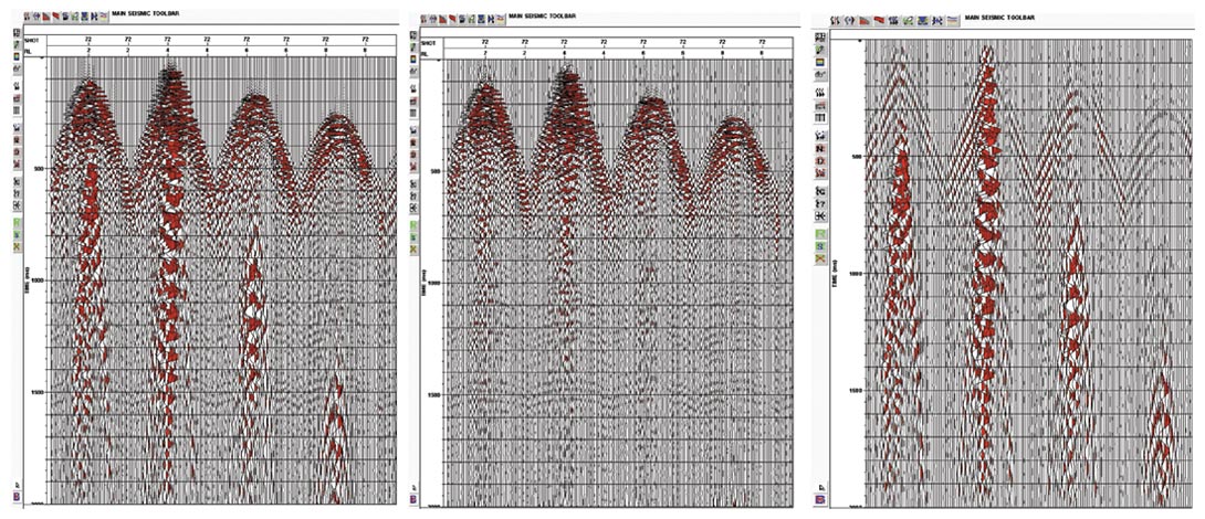
The result of the application of the described method on 2D data is shown in Figure 3.

On the left is the input data with three zero traces inserted after each original; in the central panel, we see the result after interpolation; and finally, on the right we show the difference between input and output traces at the original positions. Note, that the method was able to interpolate dipping events (ground roll).

Figure 4 shows that the amplitude behaviour is preserved after two times upsampling, which is important if AVO analysis is to be performed after regularization.

Group interval reduced four times.
Group interval reduced two times.

Examples: 5D Regularization

Global interpolation of the 3D data is commonly referred to as 5D, because each trace in the 3D survey is defined by time and four spatial coordinates: shot X Y coordinates and receiver X-Y coordinates or any derivatives of them such as CMP coordinates, offset and azimuth or shot coordinates, inline offset, and crossline offset, and so on.

An example of 3D survey geometry before and after 5D Regularization, based on the shot and receiver coordinates is shown in Figure 5.

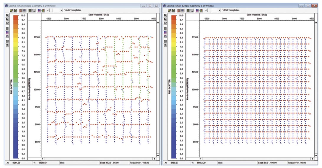
5D application on 3D data requires creating a 4 dimensional spatial grid, based on four independent coordinates and a bin size for each coordinate. Choice of these coordinates and output geometry should be based on the input geometry and regularization objectives, since the global nature of 5D Regularization always leads to creating a large amount of redundant data.

After a four dimensional grid is specified, the described method is extended to the 5D case by simply applying forward and inverse multidimensional wave number Fourier transforms at each iteration.

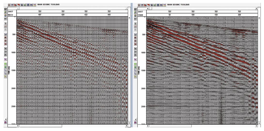
The results of 5D Regularization are shown on two 3D real datasets. Figures 6 and 7 show 5D Regularization of a very sparse survey.

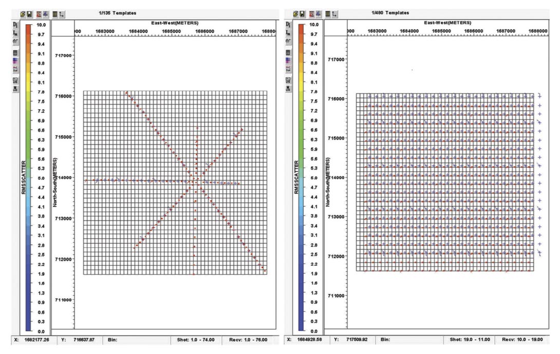
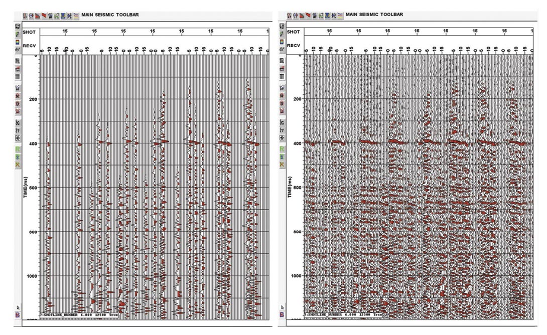
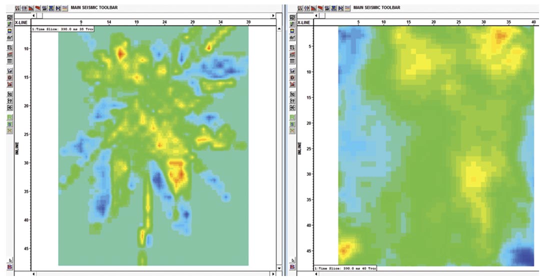
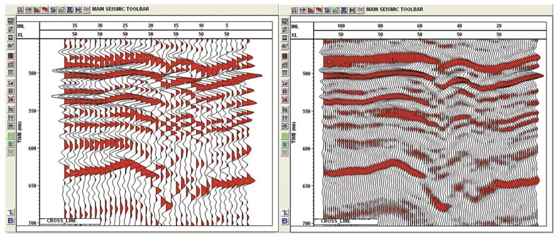
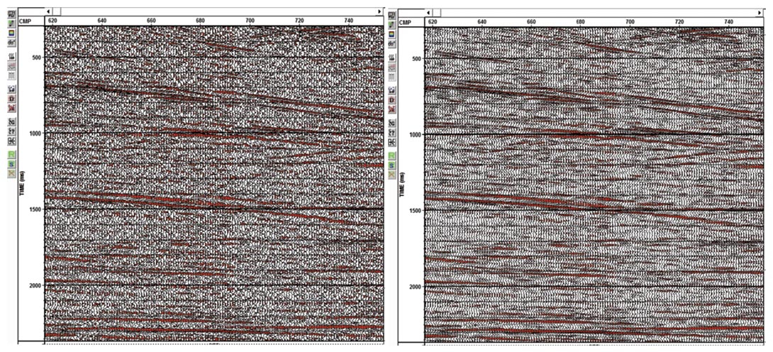
Figure 8 shows the result of 5D Regularization of a survey with diffractions and dips. The prestack time migration results before regularization is on the left and the PSTM results after three times upsampling of the prestack data is on the right. Clearly, the diffracted energy was correctly interpolated; dips and structures have been preserved and, in general, the data have become more interpretable.

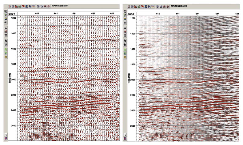
3D noise attenuation

While random noise can be effectively attenuated during the regularization process (Figures 9 and 10), we developed a separate tool to address “Ground roll” type 3D linear noise based on the same technique. In the frequency-wave number domain this linear noise has the form of a pie in the 2D shot domain and in the 3D shot domain (or the cross-spread domain) the noise takes the form of a cone. Even when noise looks separated, spectral leakage due to uneven spacing, missing traces and zero-padding always causes noise and signal mixing in the FK domain. An iterative process is employed to isolate the signal from linear noise and prevent “leaking”.

A new regular rectangular grid is created, filled with zero data and available input data. This is then converted to the frequency and two dimensional wave number domain. At each iteration, only those spectrum components bigger than a specified threshold are selected.

To isolate the signal, while leaving the noise untouched, the threshold search area of the spectrum is limited to a cone above the maximum linear noise velocity parameter and truncated at the current values of the maximum wave numbers.

Figure 11 shows the area used during this signal search.

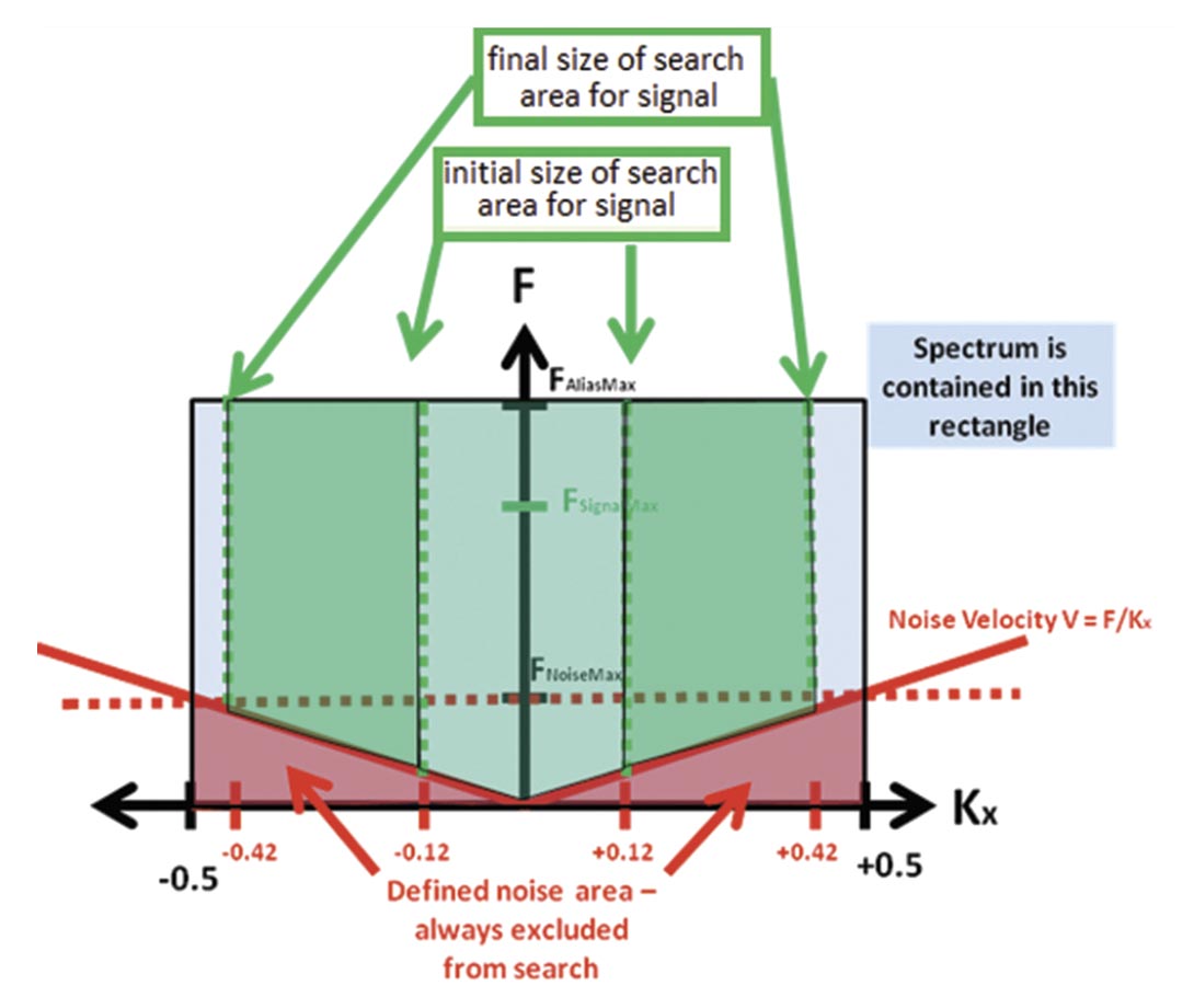
After each iteration, the threshold is reduced from the defined value to eventually reach zero at the last iteration. The maximum wave numbers, in both the X and Y directions, are also changed in a similar fashion, according to the defined start and end values. Thus, high amplitude, high velocity signal will first be selected during the iterative process.

After the iteration process is completed, the residual spectrum will contain lower frequency linear noise and also some random noise corresponding to high wave numbers.

The final residual spectrum therefore contains the linear shot noise we are trying to remove. Hence we simply subtract this from the original data or, optionally, we can use adaptive subtraction.

An important part of preserving the signal is that only noise was regularized during this iterative process.

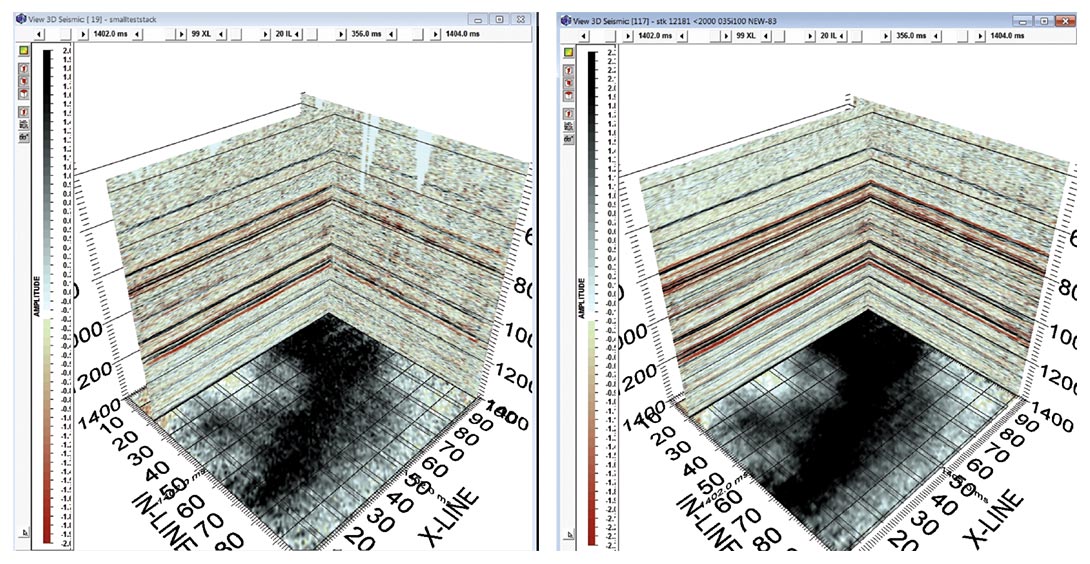
Figure 12 shows the 3D linear noise subtraction results with the difference plot on the right, proving that no high velocity signal has been removed.

Reliability of regularization and future development

Although the results can look impressive, there is always a question “Can we trust it?” or “How to pick parameters” to make regularization reliable and suitable for our purposes.

It is becoming common practice, subsequent to the regularization procedure, to use the difference between input traces and new traces at the same position to estimate quality. This difference cannot, however, be used to predict quality “a priori”.

Our current active research is focussed on the creation of a tool to estimate regularization parameters, based on the input data velocities, frequency content and input and output geometry.

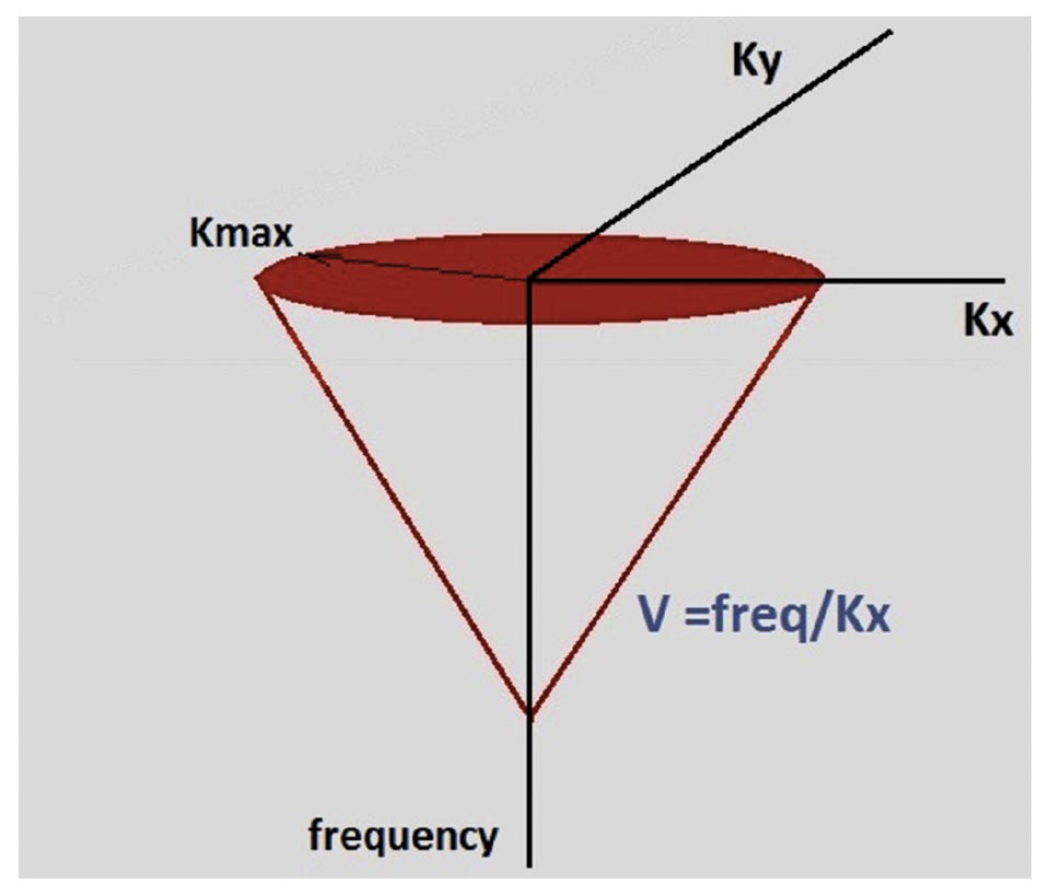
The red cone in Figure 13 represents input data in the frequency- Kx-Ky domain, limited to the defined minimum velocity we wish to interpolate.

Therefore, for any frequency (e.g. dominant or maximum) it will be a circle with the centre at K=0 and known radius Kmax, defined by the formula:

Kmax = frequency / V min

In the 5D case this area will have the form of a 4-dimensional sphere.

We assign values 1 to the “red” signal area and zero outside the circle.

Knowing input and output geometry, we create a 4- dimensional sampling operator, consisting of “ones” at the original trace positions and “zeros” everywhere else.

Now this sampling operator can be convolved with the circle (or rather 4D sphere) to estimate spectrum interference for the defined frequency and minimum velocity.

In adjusting these parameters one can best decide on how to interpolate each particular dataset.

The same approach can be used during 3D seismic survey planning with subsequent regularization in mind.

Conclusions

In spite of the common misconception, that regularization in the frequency-wave number domain is unsuitable for upsampling, we have shown that, with proper handling of the frequencywave number spectrum, Fourier domain regularization is a powerful tool to interpolate sparsely populated surveys, to upsample seismic data with diffractions and dips as well as suppress random noise.

Finally, based on multi-dimensional Fourier domain regularization, an effective 3D linear noise attenuation technique has been developed.

Acknowledgements

I would like to thank Mike Galbraith, GEDCO for initiating and supporting this work.

Special thanks to Alan Richards, Edge Technologies Inc., Calgary for his invaluable input.