Gabor Deconvolution: extending Wiener’s method to nonstationarity

Summary

Seismic data is arguably always nonstationary in its Fourier spectral character since anelastic attenuation processes are present everywhere. The major mathematical tool for dealing with this effect in seismic data processing is the Wiener deconvolution algorithm, which is at least a half century old. Paradoxically, this algorithm assumes that the seismic time series is stationary. Nevertheless, Wiener’s algorithm deals with a limited class of attenuation effects in an average sense. When posed in the Fourier domain, the algorithm suggests its own generalization using a nonstationary extension of the Fourier transform such as the Gabor transform. A simple computational scheme for the Gabor transform is presented that is based on a set of windows that form a partition of unity. The use of the Gabor transform in a nonstationary deconvolution scheme is enabled because it factorizes the nonstationary convolutional model for a seismic trace with attenuation. The Gabor transform of a seismic signal is shown to be given approximately by the product of the Fourier transform of the source signature, the time-frequency attenuation function, and the Gabor transform of the reflectivity. Gabor deconvolution smoothes the Gabor magnitude spectrum of the seismic signal to estimate the product of the magnitudes of the attenuation function and the source signature. A phase function is then estimated using the minimum phase assumption. The result is a complex-valued, time-frequency function that we call the spectrum of the propagating wavelet. When the original Gabor spectrum is divided by this time-frequency spectrum of the propagating wavelet, the result is an estimate of the Gabor spectrum of the reflectivity. Testing on nonstationary synthetic signals shows that Gabor deconvolution is dramatically effective in producing a very broadband reflectivity estimate, far better than Wiener’s algorithm. Testing on real data also shows very highly resolved images from Gabor deconvolution. When compared with a “standard” image created using surface-consistent Wiener deconvolution together with time-variant spectral whitening, the Gabor images show subtle enhancement of detail and greater robustness in the presence of coherent noise and coverage gaps.

Introduction

Norbert Wiener’s deconvolution algorithm, brought to geophysics by the legendary Enders Robinson and Sven Treitel (Robinson and Trietel, 1967, and Peacock and Trietel, 1969) is both elegant and hugely important. In a simple prescription, it tells us how to whiten and phase-correct seismic data. Underlying this algorithm is the convolutional model of a seismic trace, which is usually stated by postulating that the seismic trace is the convolution of two other signals, one which we call the “wavelet” and another that we call the “reflectivity”. Wiener deconvolution adopts this convolutional model and proceeds to make assumptions about both wavelet and reflectivity in order to estimate and remove (i.e. de-convolve) the former, thus revealing the latter. Plausible though this model is, it does not accommodate many physical effects such as attenuation and the general multiple series. For this reason, we have developed a nonstationary extension of the convolutional model and use it as the basis for a new deconvolution technique that directly estimates and removes both Q attenuation and source signature. The initial work on this new algorithm was presented at the 2002 CSEG National Convention (Margrave and Lamoureux, 2002).

A Nonstationary Convolution Model

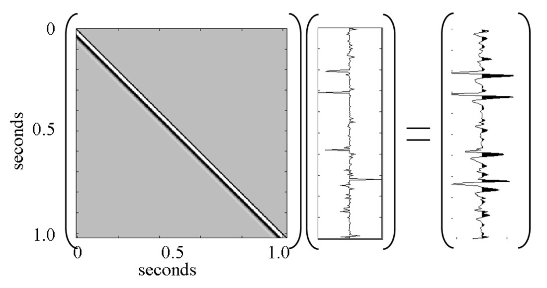
Figure 1 illustrates the stationary convolutional model by showing a source waveform being convolved with a reflectivity time series. Thus we are modelling no multiples or attenuation other than those that can be considered as part of the effective source. The convolution is achieved by constructing a special matrix containing the source waveform and multiplying it into a column vector containing the reflectivity. In the convolution matrix, the source waveform appears in each column with its first sample shifted to lie along the main diagonal. This results in a matrix where every diagonal (from upper left to lower right) has a constant entry. This symmetry is called Toeplitz and is the telltale sign of a stationary process.

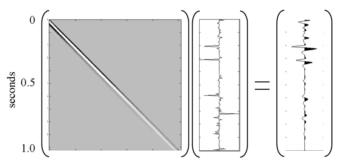
In contrast, Figure 2 shows a nonstationary replacement process in which the same reflectivity as Figure 1 is being acted upon by a matrix that represents a nonstationary attenuation process. Each column of the nonstationary convolution matrix contains the effective source for the time corresponding to the main diagonal. From upper left, representing early times, to lower right, representing later times, the effective source waveform shows a steady decay in both amplitude and frequency due to the attenuation mechanism. When applied to the reflectivity column vector, the result is a very different seismogram from Figure 1 and shows a progressively attenuated response. This is a nonstationary convolutional model that is formulated to include the effects of attenuation wherever it may occur. (This model was suggested earlier by Schoepp and Margrave, 1998).

The matrix operation shown in Figure 2 is most conveniently expressed as a mathematical form known as a pseudodifferential operator. This somewhat intimidating term is really nothing more than a nonstationary filter (Margrave 1998) that proceeds exactly as discussed in the preceding section. Formally, we can represent Figure 2 by the equation

In this equation, the integral is taken over all time, t and f are time and frequency, r is reflectivity, w is the source waveform, s is the seismic trace, a “hat” over a variable indicates the (forward) Fourier transform, and α is the time and frequency dependent attenuation function. In the case of the commonly assumed “constant Q” model (Kjartansson, 1979), α is given by

in which H denotes the Hilbert transform. The stationary convolutional model emerges as a special case of equation (1) corresponding to infinite Q. In this case α=1 and the integral in equation (1) becomes an ordinary Fourier transform giving

which we can recognize as the standard convolutional model since multiplication in the frequency domain is convolution in the time domain. (The subscript on s in equation (3) is to distinguish the stationary signal from the nonstationary by reminding us that the former corresponds to Q=∞.)

Equation (1) is structured to prescribe the Fourier transform of the seismic trace rather than the trace in the time domain because it is mathematically simpler. When this equation is rewritten in the time domain and specialized to discretely sampled time series with particular values for the parameters, the representation shown in Figure (2) results.

The Gabor Transform

We now present a solution of the nonstationary deconvolution problem as posed by equation (1). An essential tool in our solution algorithm is an extension of the Fourier transform known as the Gabor transform. Originally proposed by Dennis Gabor (Gabor, 1946), the inventor of the hologram, as a tool in quantum mechanics, the Gabor transform uses a window function to localize a signal to a certain time range and then applies the Fourier transform. Sometimes called a short-time Fourier transform, the Gabor transform uses a suite of windows designed to allow the process to be invertible. Gabor initially suggested using Gaussians as window functions but the theory has evolved since then to allow a great variety of windows (see also Bastiaans, 1980, Feichtinger and Strohmer, 1998, Grochenig, 2001).

We have developed a particular implementation of the Gabor transform, appropriate for discretely sampled, bandlimited signals based on the concept of a partition of unity (POU). APOU is a set of windows defined on the real line and so chosen that they always sum to unity. If Ω(t)>0 denotes an always positive window function, then it forms a POU if

where by Ω_n we mean the window Ω translated (shifted) to the time nΔt. The POU defined by equation (4) uses a single window function translated at regular intervals along the real line to form a POU. This is simple and convenient but not necessary. The windows of a POU need not be formed from translations of a “mother” window, they just need to sum to unity.

Next we define an analysis window, g, and a synthesis window, γ, by the equations

and

So g and γ are just fractional powers of Ω such that

We define the Gabor slice using the analysis window g as

and the Gabor transform is the Fourier transform over the set of Gabor slices

This equation emphasizes that the Gabor transform of s is a two-dimensional time-frequency decomposition. Here time is denoted by the integer n and frequency by the real number f. The use of a continuous variable for frequency is just a notational convenience as, in any numerical implementation we use the discrete Fourier transform and calculate equation (9) over a discrete set of frequencies as well as times.

The inverse the Gabor transform is easily accomplished using the synthesis window γ, the inverse Fourier transform, F-1, and summation over n, by the equation

That this recovers s exactly follows because the inverse Fourier transform recovers the Gabor slice (equation (8)) and the summation over n using equation (7) recovers s.

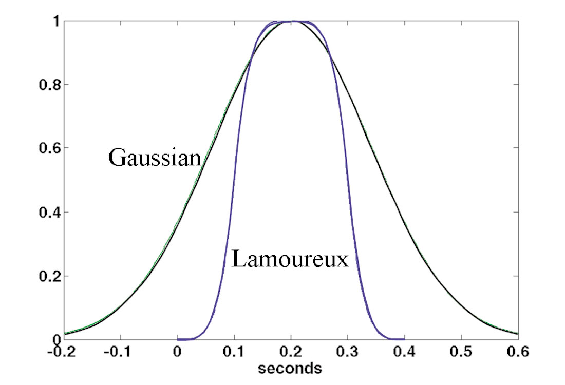
Figure 3a illustrates the Gabor spectrum of a synthetic seismogram constructed using the nonstationary trace model of equation (1). The Gabor spectral plot shows only the magnitude of G[s] and black indicates a large positive value while neutral grey is a very small number. The Gabor spectrum shows clear decay in both time and frequency. Also evident are the imprint of the reflectivity and the bandlimiting due to the source waveform.

Factorization of the Nonstationary Trace Model

In a complicated technical result that we will not reproduce here, we have shown that when the Gabor transform is applied to the nonstationary trace model proposed in equation (1), the result is approximately a product of factors that is analogous to equation (3), given by

where the ellipses indicate the presence of further terms required to make equation (11) an equality. (Since equation (1) gives the Fourier transform of our trace model, we must first apply the inverse Fourier transform to equation (1) before applying the forward Gabor transform.)

We will not present the detailed mathematical justification of equation (11) here; but, it is easy to see why this result makes sense. Isolate a small portion of a seismic trace with a window; then, from the perspective of the stationary convolutional model, we expect its Fourier spectrum to factor into the product of an effective wavelet (Fourier) spectrum times a reflectivity (Fourier) spectrum. Now, if we repeat this process for the same window shifted to a later time, we expect the Fourier spectrum to be the product of the spectra of a different effective wavelet and a different reflectivity. If we consider only attenuation and neglect multiples, then these two different effective wavelets are both the product of the Fourier spectrum of the actual waveform emitted by the source times a different Q filter for each window position. That is precisely what the first two factors on the left-hand-side of equation (11) are. Then, having a different reflectivity spectrum involved in each window is precisely what is meant by having the third factor since the Gabor transform is simply a windowed Fourier transform. In this light, for fixed n, equation (11) is simply a temporally localized version of the stationary convolutional model. The explicit appearance of the attenuation function and Gabor transform of the reflectivity simply provides the connection between different windows.

The preceding paragraph explains why equation (11) is precisely what should be expected from localizing the stationary convolutional model; but perhaps we should say why it is not an exact factorization of equation (1). The approximations come in two places, first we have represented the Q filter by its value at the window centre instead of allowing it to vary continuously across the window. Second, while the form of the windowed seismogram is mostly controlled by the reflectivity within the window, there is always some non-local effect from outside the window. Since the wavelets involved are minimum phase, the non-local effect should be entirely from earlier times.

The Gabor Deconvolution Algorithm

We now assume that equation (11), without any implied error terms, is a precise description of the Gabor transform of a seismic signal. Furthermore, we will find it convenient to assume that the attenuation function is of the form given by equation (2). This is an assumption of minimum phase since equation (2) has the property that the phase of α( t,f ) is given by the Hilbert transform of the logarithm of the magnitude, |α( t,f )|, where the Hilbert transform is taken over f at constant t. We also assume that the source waveform, w(t), is minimum phase.

A virtue of the nonstationary spectral factorization of equation (11) versus the stationary factorization of equation is that the former has a clear separation of source waveform and the attenuation process. If equation (3) is to be valid then the source waveform must include an attenuation term, but there is no apparent way to separate these. In the nonstationary factorization, the source waveform is a function of f only while the attenuation function depends upon both t and f. In fact, if Q is constant, then according to equation (2), |α( t,f )| should be constant on the hyperbolic family tf = constant.

As in stationary deconvolution, we also assume that the reflectivity is a random sequence though precisely how this manifests in the Gabor domain is not clear. In a practical statement, we assume that the detail in G[s](n,ƒ) is due to G[r](n,ƒ) while the general trends are due to ŵ(ƒ)α(n,ƒ). This implies that there exists some smoothing or fitting operation that can separate G[s](n,ƒ) into detail and trend and so estimate ŵ(ƒ)α(n,ƒ) and G[r](n,ƒ).

As with Wiener deconvolution, the first step in our algorithm is to discard the phase by taking the magnitude of G[s](n,ƒ). We then apply some sort of smoothing operation whose goal is to eliminate all features attributable to G[r](n,ƒ). We have experimented with various smoothers and least squares fitting. The simplest possible smoothing procedure is to convolve the Gabor magnitude spectrum of the seismic signal with a 2D boxcar, whose time and frequency dimensions must be chosen empirically. A major problem with this approach is that it has an amplitude equalization effect, much like an AGC, that tends to distort the estimated reflectivity. Usually better is a technique we call hyperbolic smoothing. Since the level-lines of the attenuation function, for Q a constant, are the hyperbolic family defined by tf = constant, we are motivated to calculate the mean value of the Gabor magnitude spectrum along such contours. In this case, we take the mean along hyperbolic contours as an estimate only of |α(n,ƒ)|. We then divide |G[s](n,ƒ)| by the estimate for |α(n,ƒ)|. The result of this division is averaged over t and smoothed in f with a convolution operator to estimate |ŵ(ƒ)|. Another possibility is to perform a least-squares fit of the model of equation (11) to G[s](n,ƒ).

In any case, assume for the moment that a particular smoothing or fitting operation has been conducted on G[s](n,ƒ). This becomes an estimate of the Gabor magnitude spectrum of the propagating wavelet that we will call |ŵ_α| and we assert that

where the approximation holds with a hopefully small, but admittedly unknown, error term. We then invoke the minimum-phase assumption to calculate the phase of ŵ_α. With the inclusion of a small stability constant ε, as in Wiener deconvolution, we estimate the entire Gabor spectrum of the propagating wavelet as

where we understand that both sides of the equation depend on discrete time n and frequency f, and the Hilbert transform is to be taken over frequency.

Having completed an estimation of the Gabor spectrum of the propagating wavelet, we now perform the actual deconvolution by spectral division in the Gabor domain

where we have used s_d to symbolize the deconvolved seismic trace and the division is understood to be a point-by-point operation using complex arithmetic. s_d itself is recovered by an inverse Gabor transform of the result from equation (14). Usually, it is convenient to bandlimit G[s_d](n,ƒ) in the Gabor domain prior to the inverse transform. Since the attenuation function may be nearly constant along the hyperbolae tf = constant, we find it suitable to define a (time-variant) high frequency cutoff whose value follows a particular hyperbolic trajectory.

We now begin an example of the process starting with the synthetic signal and its Gabor (magnitude) spectrum shown in Figure 3a. This synthetic signal was created with equation (1) using a Q of 40, a minimum-phase source signature with a dominant frequency of 20 Hz, and a computer-generated random reflectivity. Figure 3b shows the estimate of |ŵ_α| calculated by hyperbolic smoothing. We do not show the corresponding minimum-phase spectrum that is calculated as the Hilbert transform of the natural logarithm of |ŵ_α|. In Figure 3c we show the result of the spectral division of equation . The Gabor spectrum, whose magnitude is shown in Figure 3a, was the numerator and that of Figure 3b was the denominator. This is an estimate of G[r](n,ƒ) and has been high-frequency limited along a hyperbolic trajectory between 1 and 2 seconds and along a vertical trajectory above 1 second. The rather startling detail in Figure 3c is invisible in Figure 3a because it corresponds to amplitudes too small to be displayed with the dynamic range of the grey scale. For comparison, Figure 3d shows the actual G[r](n,ƒ) without bandlimiting. While there are many similarities in the details of Figures 3c and 3d, there are also differences. It may be possible to improve this result with a better procedure for estimating |ŵ_α|; but, at present this is the best that we can do.

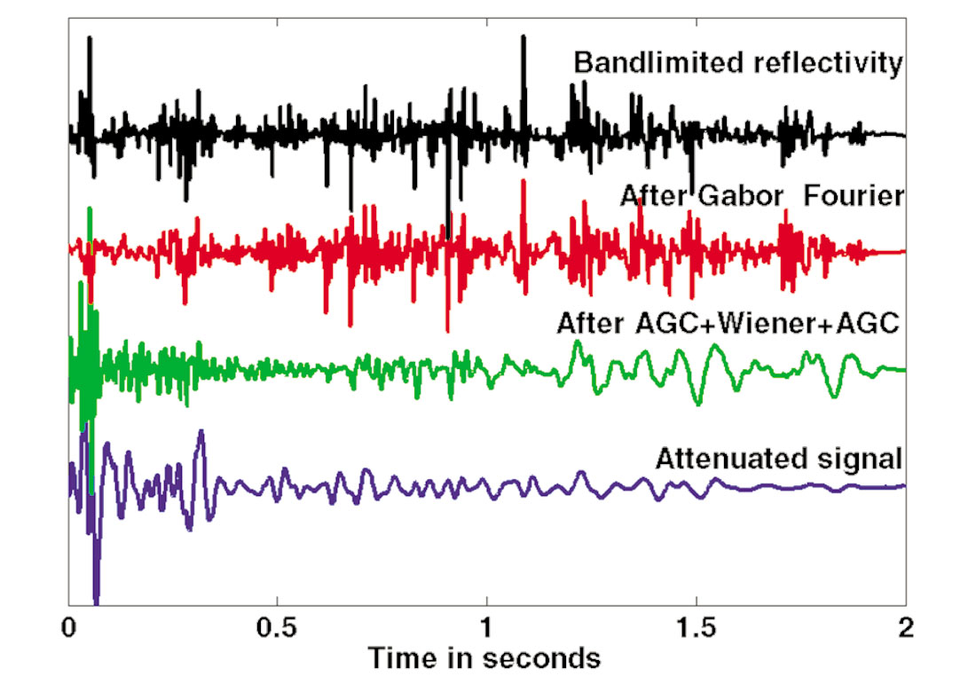
Figure 4 shows time-domain traces which are (from the bottom up) the input attenuated seismogram, the Wiener deconvolution result, the Gabor deconvolution result, and the bandlimited true reflectivity. (The reflectivity was given the same bandlimit as the Gabor spectrum show in Figures 3c). Thus, the bottom trace was input directly into Gabor deconvolution and the result is the third trace from the bottom. In comparison with the answer (at top) the Gabor deconvolution result has estimated a very high resolution reflectivity that has a strong correlation with the answer. We emphasize that this was done without knowing the value of Q. The Wiener deconvolution result is also interesting. Clearly this deconvolution assignment was a task well outside the design assumptions of the Wiener algorithm. However, so also is the task posed by real seismic data. Close inspection of the Wiener result in the design gate (.8-1.2 seconds) shows that it is a reasonably good result there, with some resolution of the major events. However, even over this design gate, where the result should be ‘optimal’ there is clear evidence of spectral decay. At earlier times, there is evidence of overwhitening and also there is obvious underwhitening (poor resolution) at later times.

Compact Gabor windows for Computational Efficiency

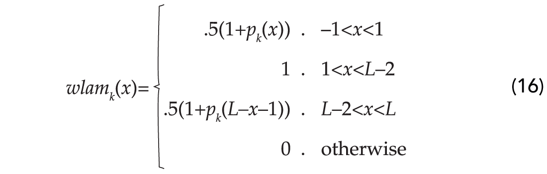
As an alternative to the Gaussian window suggested by Gabor, we have adopted the use of the window shown in Figure 5, which we call a Lamoureux window. The elementary Lamoureux window reaches unity at a single central point and is a polynomial on either flank. The flanks are chosen such that a point that is δt from the beginning of the window has amplitude say a and the point that is δt from the central peak has amplitude 1–a. This property allows an easy construction of a POU. A smooth window is found by choosing the unique odd polynomial of degree 2k+1 which has its first k derivatives equal to zero at x=1, and satisfies p_k(1)=1, then shifting and glueing together these pieces. For instance, such polynomials are given as

and the corresponding Lamoureux window is given by

In comparison with a Gaussian window of the same width, the Lamoureux window is much more localized. (The width of the Gaussian is defined as its 1/e point.) In the context of the theory of the Gabor transform, if we choose p=1/2, then we will actually window with the square root of the Lamoureux window in both analysis and synthesis. For this reason, a 4^th order Lamoureux is a natural choice so that the window can approach zero as a 2nd order curve. In contrast, if we used the popular raised cosine window, then the fact that its square root approaches zero linearly and has discontinuous slope at its endpoints could lead to undesirable manifestations such as spectral ringing.

The use of compactly supported windows leads to great efficiencies in the Gabor transform. When using Gaussian windows, each windowed trace segment is as long as the original trace. So if n windows are required and the trace is of length N, then the computation effort is proportional to nNlog₂N. In contrast, if the compactly supported window is of length M where M is typically 0.1N or less, then the effort is nMlog₂M≈ .1nNlog₂N. So we expect at least an order of magnitude less effort.

When using Gaussian windows, the window width and increment are essentially independent. In contrast, to form a simple POU with Lamoureux windows, the window spacing is determined by the width because the adjacent windows must have their peaks over the endpoints of the window in Figure 5. This is a minimally redundant POU (redundancy of 2). However, we can overcome this apparent obstruction to more redundant representations by simply shifting the minimally redundant partition by, say, 1/2 a window width, and merging the shifted partition with the original partition. By this scheme, we can achieve any integral redundancy.

Real data comparison

We now present a comparison with real data. Most of the data processing was not done by us, but rather by Sensor Geophysical of Calgary, Alberta. Sensor has a reputation as an excellent, technically sophisticated data-processing shop that specializes in very high resolution images. Their standard processing flow, developed with a great deal of careful study and experimentation, is highly sophisticated, and we only comment on the steps required for comparison with Gabor deconvolution. Sensor’s standard flow begins with true-amplitude gain recovery and continues with surface consistent Wiener deconvolution. This is followed by TVSW (time variant spectral whitening), CMP Stack, TVSW again, and FX noise reduction. TVSW is an interesting process that does a strong, nonstationary spectral whitening that is effectively zero phase. The algorithm essentially uses a POU (partition of unity) in the Fourier domain to specify a set of narrow band filters that break a signal into a given number of frequency slices. These filters are chosen to span the expected signal band and typically have a 5 or 10 Hz width. Since the filter’s spectral shape is based on a POU, the frequency slices sum to recover the original signal. The TVSW process runs an AGC on each filter slice (in the time domain) and then sums them. This process has many virtues including rendering the amplitude spectrum essentially stationary, trace balancing, and coherent noise suppression.

Though not obvious, the results are very similar to running Gabor deconvolution using a box car smoother and associating a zero phase spectrum with the |ŵ_α| estimate. For comparison, we substituted a pre-stack Gabor deconvolution for the sequence “true-amplitude recovery, surface consistent deconvolution, and TVSW” and replaced the post-stack TVSW with a post-stack Gabor deconvolution.

Rarely in seismic data processing is a comparison of processes without secondary complications. We have several here. First, we found that we could recover a much broader signal band with Gabor deconvolution than was attempted with the standard processing. The standard processing recovered signal out to about 125 Hz while we found that we could push this number to 160 Hz with Gabor deconvolution (this is 2 mil data so the Nyquist frequency is 250 Hz.). At this time we do not know whether the standard flow could be pushed higher. Another complication is that we chose to insert radial-trace filtering in the Gabor flow because we hoped to demonstrate recovery of reflection signal at very low frequencies. The radial-trace filtering process is very effective at removing coherent source noise which might allow the low-frequency reflection signal to be recovered. We are still assessing this point and will not report further on it here.

We have not done a great deal of parameter testing. The Gabor algorithm has several important parameter choices including the selection of window type (Gaussian or Lamoureux), window width, window spacing, choice of “p” value in equation , smoother algorithm and smoother lengths, and white noise level. For this case we chose Lamoureux windows of .2 seconds long, 50% window overlap, p=.75, hyperbolic smoother with a 10 Hz frequency boxcar, and a white noise level of .0001 . It may well be that different parameter choices could provide superior results than shown here though we have found the algorithm to be quite robust with the parameters as given.

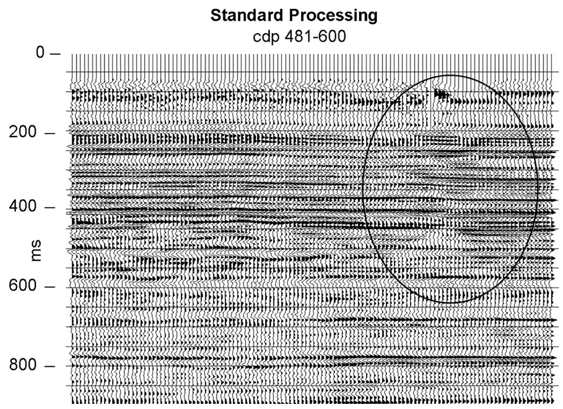
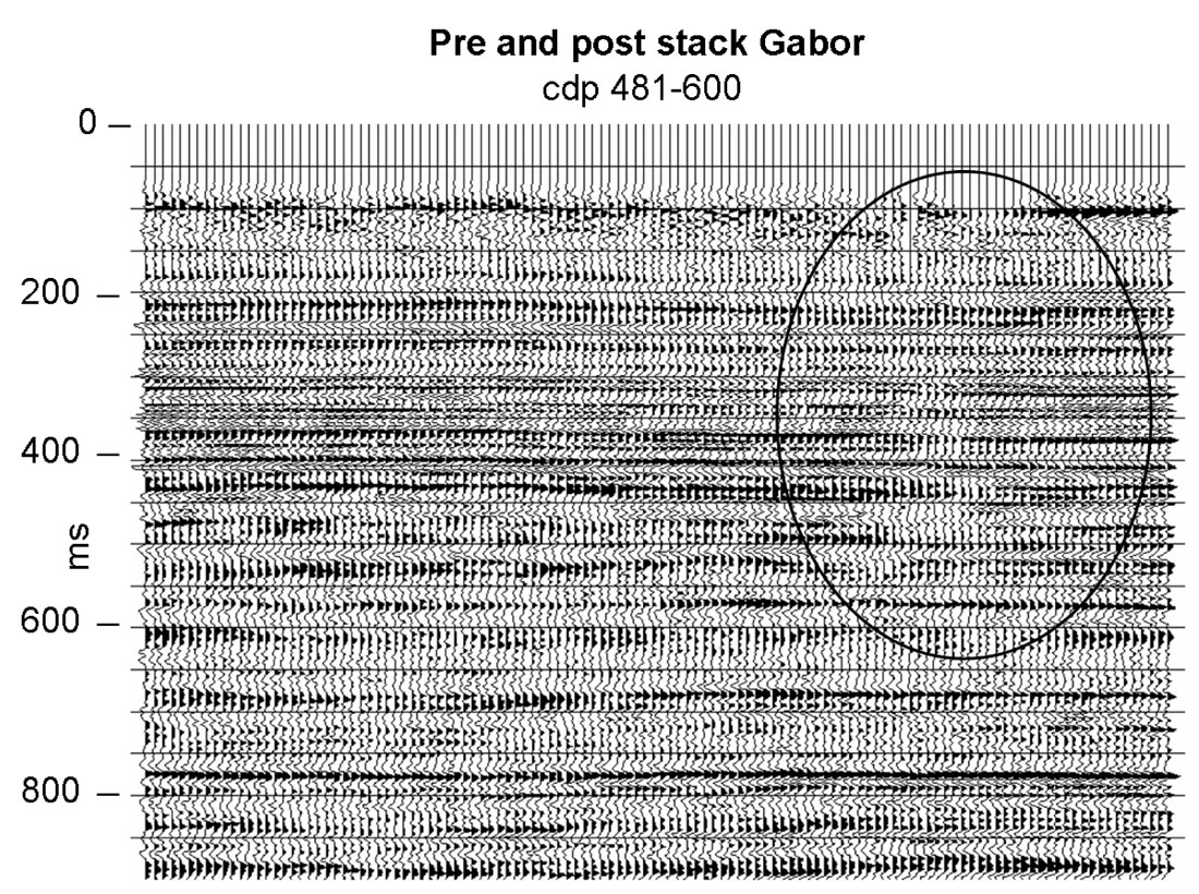
Our test line was provided courtesy of Husky Energy and was acquired over a sedimentary basin using a dynamite source. Figures 6 and 7 show CDP’s 481-600 of our seismic line processed by the standard flow and the Gabor flow, respectively. The bandwidth of the Gabor result is visibly greater, even at this display scale (and the residual random noise is somewhat greater, as well). The overall amplitudes of the Gabor result are more uniform in time than the standard result, indicating possibly too much amplitude levelling caused by two passes of the Gabor algorithm. We conjecture that this effect could be lessened by choosing alternative parameters in the post stack Gabor. The highlighted feature is a small gap in surface coverage, which seems to be effectively ‘healed’ by the Gabor processing. The single-channel nature of our Gabor code means that it is rapidly adapting spatially as well as temporally. Surface-consistent deconvolution, in contrast, is constrained to change quite slowly. Amplitudes of most events appear more laterally consistent on the Gabor result than on the standard version, even though the Gabor result is greater in bandwidth.

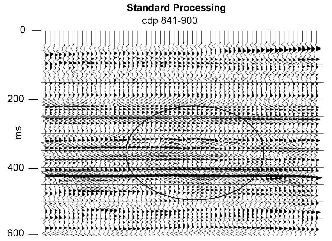
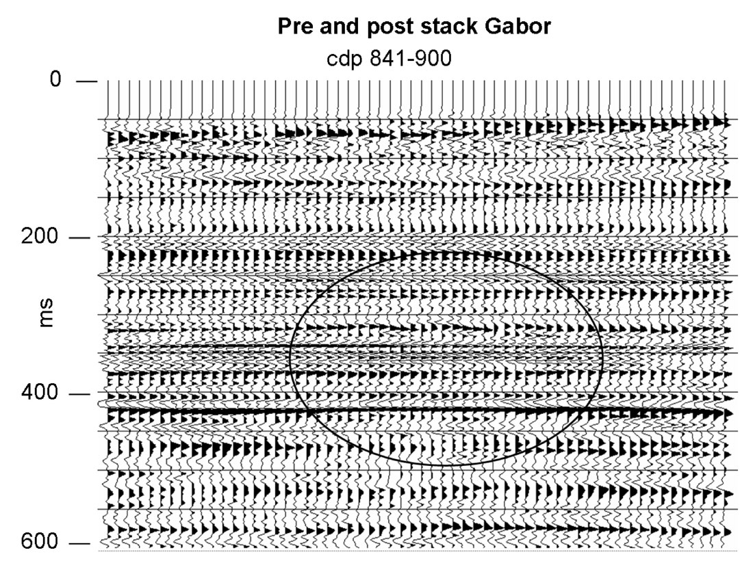
The outlined feature in Figures 8 and 9 is likely a geological anomaly. It is more precisely delineated by the increased bandwidth of the Gabor result. In addition to greater bandwidth, the Gabor result appears to have better lateral continuity.

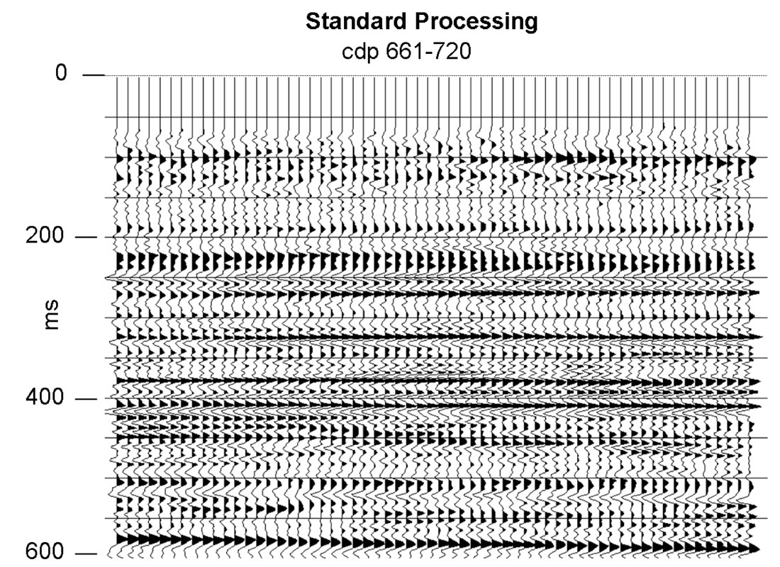
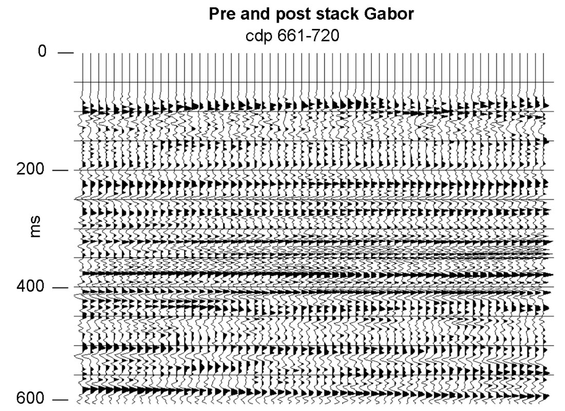
Figures 10 and 11 show CDP’s 661-720. The Gabor result has visibly greater bandwidth without any sacrifice in continuity. For example, note the doublet event whose bottom loop is right on 350 ms on the right hand side of the Gabor result. This event is continuous across most of the section but is really not discernable on the standard result.

A VSP experiment

With the evidence in the previous section, it might be concluded that Gabor deconvolution gives an incrementally higher resolution image than the standard flow. However, the validity of that image may still be doubted. As an additional test, we conducted an analysis of a unique dataset provided to us by Encana. This consisted of 5 surface vibration points at various offsets from a well with 3C receivers in a surface spread and in a VSP configuration downhole. Each sweep was recorded simultaneously into both receiver arrays.

We followed standard practice to perform wavefield separation on the VSP in order to directly estimate the downgoing waveforms. We then estimated the apparent waveforms in the surface data using three different methods: Gabor deconvolution, timedomain Wiener deconvolution, and frequency-domain Wiener deconvolution. The Wiener methods were done on gained data in temporally short analysis windows that were moved down the traces in increments. These were the same windows used by Gabor deconvolution. The Gabor estimates were made on raw data. At this point, we had wavelets observed in the VSP as a function of depth versus those observed on the surface as a function of two-way traveltime. These are not directly comparable since the VSP-observed wavelets have only travelled half of the travelpath of the surface-observed wavelets. Therefore we estimated Q values from the VSP using spectral ratios and developed a forward Q filter to apply to the VSP-observed wavelets to simulate travel along the two-way path to the surface.

Figure 12 typifies our results. In all cases, we observed that the Gabor estimates agreed quite closely with the direct VSP observations. While the Wiener estimates were close to one another, they differed significantly in amplitude and phase from the other two, especially in the deeper window. While the amplitude effects are simply attributable to the Wiener methods requiring gained data, the phase differences are not. In any case, without overly criticizing the Wiener results, it is pleasing that the Gabor results agree so closely with the VSP observations.

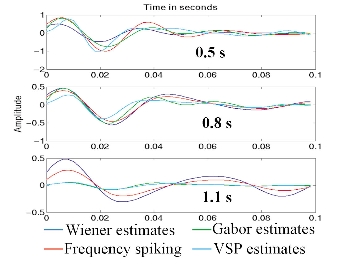
One final note, it surprised us, given the Vibroseis source, to find that the VSP observations did not require a phase rotation to agree with the minimum phase assumptions of the deconvolution algorithms. This direct observation of apparently (or perhaps “effectively”) minimum-phase wavelets from a VSP experiment has been made by others (notably Larry Mewhort of Husky Energy) and deserves more attention than we can give it here.

Conclusions

We have presented a new deconvolution algorithm that extends the standard Wiener algorithm to directly address nonstationarity of the propagating wavelet. Called Gabor deconvolution because it utilizes the Gabor transform, a nonstationary extension of the Fourier transform, our method is based on an extension of the standard convolutional model of the seismic trace to a nonstationary convolution. This new nonstationary convolutional model explicitly accounts for the waveform as emitted by the source and for its subsequent continuous modification by attenuation processes as it propagates. This model incorporates greater physical realism than the standard convolutional model.

We presented a simple mathematical framework for the Gabor transform of a discretely sampled, bandlimited signal. Our discrete Gabor transform recovers a signal exactly by using a set of windows that form a partition of unity. Furthermore, we can apply windows both at the analysis and at the synthesis stages.

Mathematically, our algorithm succeeds because the Gabor transform approximately renders our nonstationary convolutional model into a product of factors. This is similar to the fundamental fact that the Fourier transform factorizes a convolution integral except that the Fourier factorization is exact while the Gabor factorization is not. Our model predicts that the Gabor transform of a seismic signal is the product of (1) the Fourier transform of the waveform emitted by the source, (2) the time-frequency attenuation function, and (3) the Gabor transform of the reflectivity. Since it is the latter element that we desire to estimate, this suggests the possibility of estimating the product of the first two, which we call the propagating wavelet, and dividing by it in the Gabor domain.

Invoking the white reflectivity assumption, we argue that it is possible to develop a smoothing process that, when applied to the magnitude of the Gabor spectrum of the seismic trace, will eliminate all vestiges of the reflectivity and leave only the effects of source signature and attenuation function. We then recover the phase of these two factors by invoking the standard minimum phase assumption. Given this estimate of the propagating wavelet, Gabor deconvolution is completed by a spectral division in the Gabor domain followed by an inverse Gabor transform.

We demonstrated our algorithm on a nonstationary synthetic signal where it is clearly superior to Wiener deconvolution. We used a real data example to compare Gabor deconvolution to the common practice of surface-consistent Wiener deconvolution followed by TVSW (time variant spectral whitening). Though less compelling than with a synthetic there still seems to be a significant advantage in resolution from using Gabor deconvolution.

Finally we showed an example with real data where a seismic wavefield was recorded simultaneously into a VSP and a surface spread. Wavelets were estimated directly from the VSP using standard wavefield separation methods and compared with those estimated on the surface by Gabor deconvolution. Good agreement was found.

Acknowledgements

We thank the sponsors of both the CREWES and POTSI projects. These include a variety of industrial and government sources. We are especially grateful to Encana and Husky Energy for providing the data examples and to Sensor Geophysical for providing data processing. Some of this work was accomplished while some of the authors were in-residence at the Banff International Research Station (BIRS) for the mathematical sciences.