Geologic controls on seismic amplitudes

“This article was first published in the PESA News Resources magazine of the Petroleum Exploration Society of Australia in Oct/Nov 2011 and is reprinted with permission”.

Introduction

Seismic amplitudes (and AVO) can be used to derisk an exploration prospect; to characterise a reservoir; or to enhance production. By now, seismic amplitude interpretation should be regarded as a mature science, yet examples of its application with demonstrable business impact are rare. All too often, and usually with 20/20 hindsight, amplitude studies fall victim to pitfalls that might have been avoided.

A common pitfall is the failure to recognise non-hydrocarbon explanations for a seismic amplitude anomaly prior to drilling. Better predictions can be made using rock physics models to link geological thinking with geophysical data analysis. A key learning is that a wide variety of geologic controls can exert significant control over the seismic amplitude response.

Geologic controls on rock and fluid properties

Recently you might have noticed some high-profile wildcats in Australia that were touted as being amplitude-supported and yet came up dry. Whilst many passed on these opportunities, it is worth noting that the 4 cases (that I am aware of) were all eventually farmed down. I have reason to suspect that these amplitude anomalies might have been better explained by:

Well 1: a tuning effect;

Well 2: a high porosity sand;

Well 3: overpressures or a soft volcanic ash or tuff layer;

Well 4: a change in the bounding shale mineralogy (paralic to marine deposition).

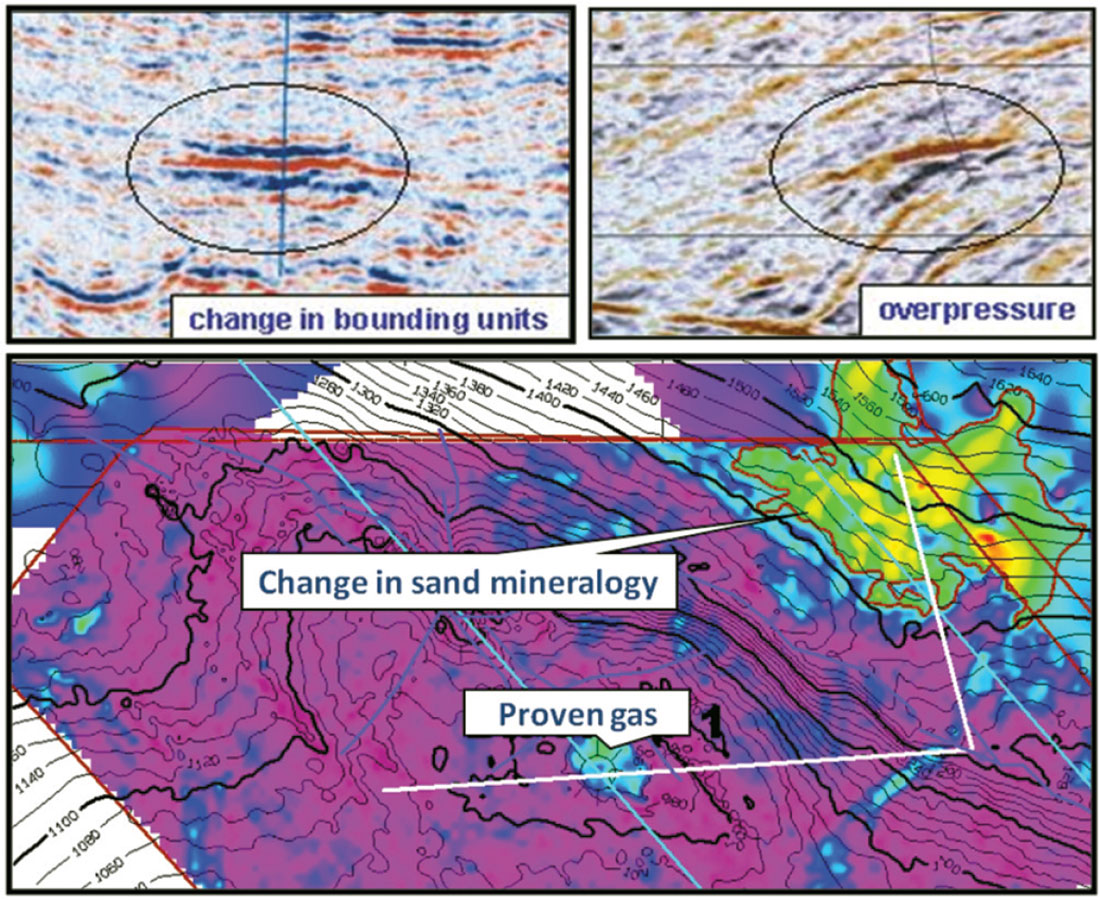
Figure 1 shows a similar story for three examples (that I can show) where amplitudes were, to some degree, touted as a reason for drilling. They highlight that it is essential to consider changes in the geology when using seismic amplitudes to derisk an exploration prospect. Of course, sometimes it may suit an explorationist to associate their prospect’s amplitude anomaly solely with the well-known “fluid effect”.

A more thorough derisking can be achieved by working though the alternative explanations using a systematic approach. Figure 2 indicates geologic parameters that may vary when attempting to predict away from well control. Frontier wildcats often target different depths, as well as different distances and azimuths to the sediment source, relative to their nearest calibration wells. The burial history of rocks and pore-fluids near the wildcat’s target depth may be vastly different to rocks and pore-fluids in the calibration wells.

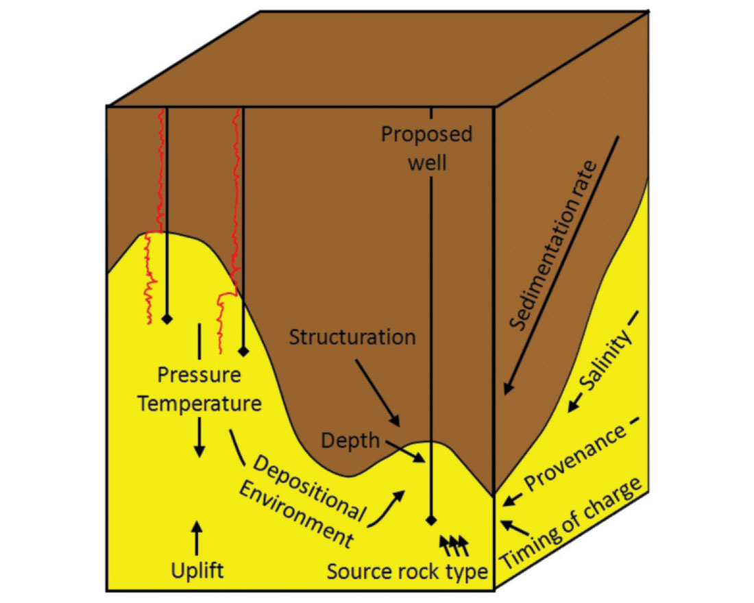
Geophysicists need to listen out for when geologists use the words shown in Figure 2 during their assessment of a prospect. The geologist’s concerns can be addressed by comparing the AVO anomaly to a collection of discrete AVO synthetics reflecting a wide range of feasible rock and porefluid outcomes at the prospect location. This is far more important than modelling with a little bit of stochastic uncertainty in the key input parameters! These synthetic models can be built by extending the available (and limited) log data using rock physics models (Avseth, et al., 2005).

Geologists need to ensure that geophysicists capture the relevant geologic controls within their favourite rock physics model. They also need to check that appropriate ranges in the rock physics parameters are tested against the seismic anomaly. This requires some knowledge of rock physics and a little bit of algebra. Don’t panic, I’m going to make it as painless as possible!

Rock and fluid property controls on seismic amplitudes

An interpretable formulation of the seismic AVO response can be made by modifying and extending the industry-standard Gassmann equations. Isotropy and low frequencies are the most significant assumptions made and are widely believed to be appropriate for traditional surface seismic. The formulation is an extension from that shown by Mavko and Mukerji (1995) and introduces the concept of shear (-wave) pore stiffness.

Its strength is that it maintains generality while reducing the analysis to as few variables as possible. Along with more elaborate rock physics models, it provides a mathematical link between the physical (and economic) characteristics of a seismically- resolvable, porous and saturated “target layer” to its elastic properties (Figure 3). These rock physical properties each depend on distinct geologic controls albeit non-uniquely, but more on this as I continue.

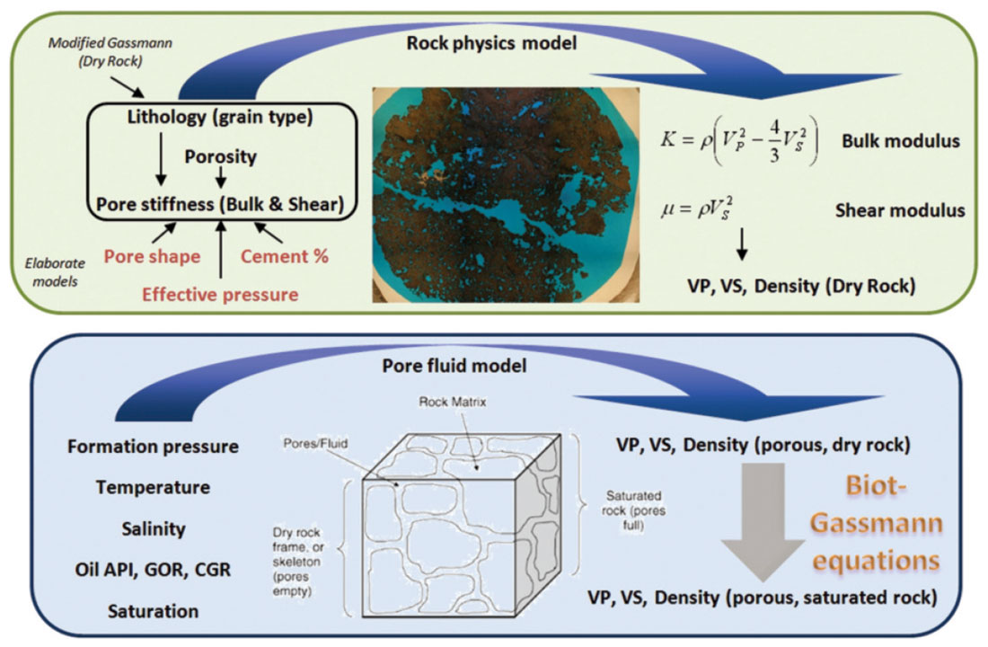
Seismic amplitudes (and AVO) depend upon the elastic properties of the target layer, which appear on the left hand side of equations 1 to 3. The rock and fluid properties all appear on the right hand side of equations 1 to 3 and these will be discussed individually in the subsequent sections. This formulation uses bulk and shear moduli (Κ and μ) instead of V_P and V_S which can be derived as indicated by equations 4 and 5.

Of course, seismic amplitudes also depend on the elastic properties of encasing layers, but I would need to introduce the complicated Zoeppritz equations (or an approximation to them) to handle that. This is done to maintain simplicity, especially because nowadays we often use seismic inversion to work with layer rather than interface properties anyway. The idea here is to focus on what controls the elastic properties (and seismic response) of one layer at a time.

Examples of non-hydrocarbon controls on seismic amplitudes

The elastic properties of the mineral component (or lithology) of a rock (Κ_Grain, μ_Grain and ρ_Grain) are linked and exert strong control on the elastic properties of the rock by virtue of their position in equations 1 to 3. Lateral variation of the lithology can be caused by a change in provenance, various diagenetic processes or via a subtle transition to a non-reservoir rock.

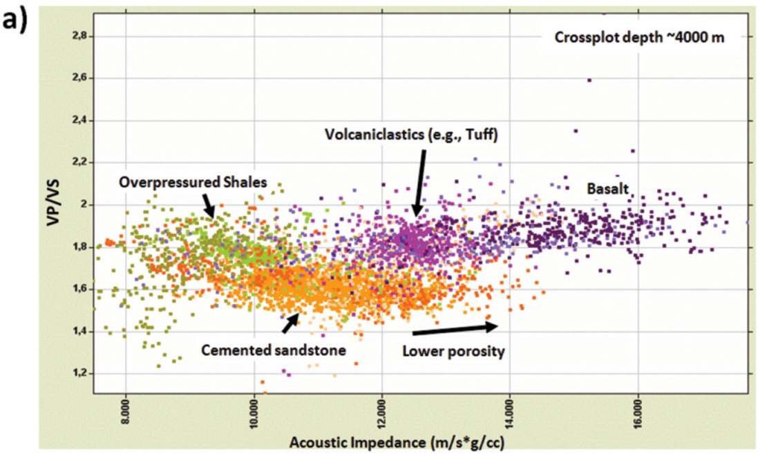
Figure 4a shows a well-log crossplot where the acoustic impedance and V_P/V_S values of 4 different lithologies are well separated and clearly different from each other. Figure 1b shows the Zoeppritz reflection coefficients generated for interfaces comprised of these lithologies. The AVO gradient appears to be a reliable indicator of reservoir (mean porosity sandstone and cemented sandstone) from non-reservoir (tuff and basalt).

Porosity also appears in equations 1 to 3 and is therefore also an important control on the elastic properties of porous rocks. Geologic reasons for porosity variation away from well control include: mechanical compaction; diagenesis; pressure solution; undercompaction; and depositional environment (i.e., grain coatings and sorting).

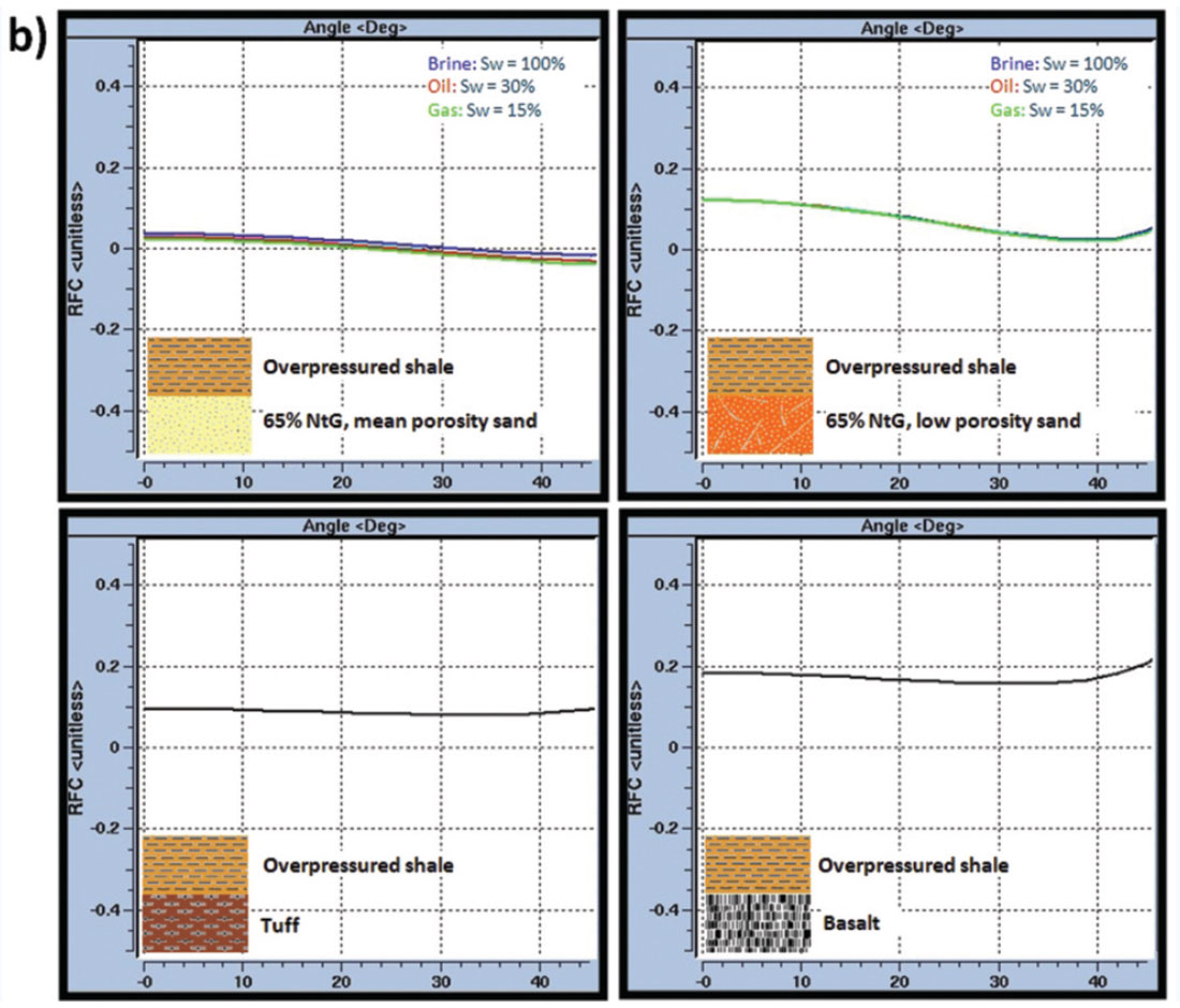
The upper panels of Figure 4b show the effect on the AVO response resulting from a 7% decrease in porosity of the sandstone halfspace. The normal incidence amplitude (or intercept) increases significantly while the AVO gradient remains similar.

the porosity is non-zero. Equations 1 and 2 contain the terms Κ_∅ and μ_∅ that represent the bulk and shear moduli of the pore space. In more elaborate models, these pore stiffnesses may depend upon pore shape (e.g., texture, fractures); the quantity of micro-scale grain-to-grain contacts; the effective pressure; the porosity and the grain properties. Their exact dependence is what distinguishes one rock physics model from another. Using equations 1 to 3 keeps things as simple as possible by lumping these potentially complicated dependencies into just two terms: Κ_∅ and μ_∅.

Figure 5 provides a striking example of pore space stiffness variability using 4 pure dolostone core plugs with similar porosities but vastly different permeabilities and different pore types (as shown in thin section). The measured shear modulus (μ_Dry) shows a large separation between many of these pore types. In carbonates, the pore type is often diagnostic of a particular facies, so if porosity can be safely constrained then this could enable carbonate facies mapping from seismic amplitudes.

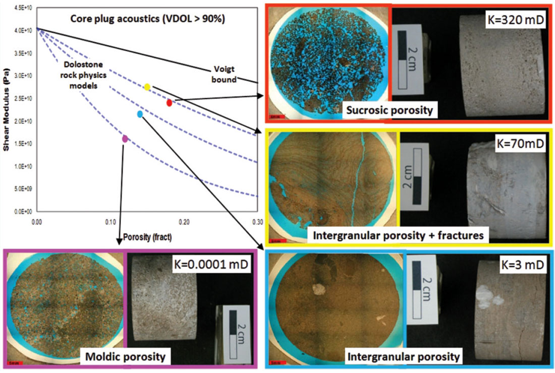
However, if the goal is to provide quantitative estimates of porosity from seismic amplitudes then the pore stiffness effect needs to be understood and heavily constrained to avoid large systematic errors. Usually this requires ample high quality log data or core acoustics, rock textural analysis and close interaction with other disciplines to assess whether pore stiffness changes could occur within the study area.

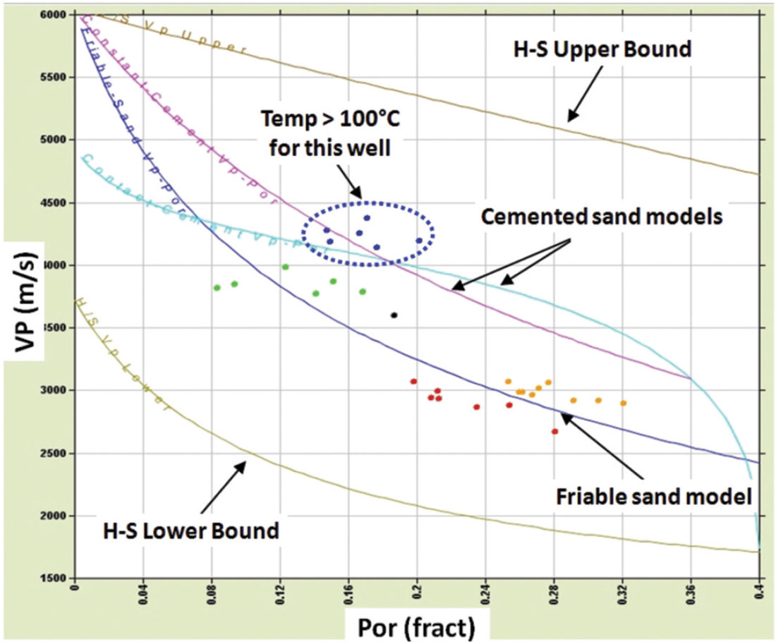
In clastic settings, this might mean studying the role of grain size and sorting on the elastic properties and using sequence stratigraphy to identify areas where the pore stiffness might change laterally. Cementation can cause sharp changes in the pore stiffness moduli, often triggered once a certain burial depth (and temperature) is exceeded (Figure 6). Petrology and basin modelling can be helpful at predicting how and where this might occur.

In carbonates, cementation usually occurs soon after burial but the rock can then undergo a wide variety of processes (dissolution, diagenesis, fracturing, a.o.) that affect pore stiffness and ultimately create a range of carbonate pore types and pore stiffnesses.

Knowledge of carbonate depositional environments and facies associations is therefore essential.

It is well known that overpressuring can affect seismic velocities. Changes in the effective pressure can act to load or unload the rock frame and in doing so influence the pore stiffness terms. Overpressuring caused by rapid burial can also act to maintain higher porosities than would be expected from mechanical compaction at a given depth. A variety of thermal effects, uplift and even hydro-geologic effects can also give rise to overpressures (Swarbrick, et al., 2002).

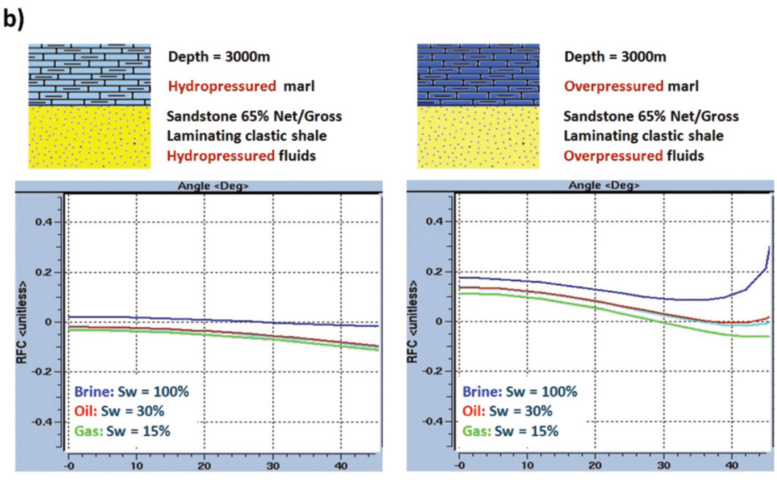
Understanding pressure effects on the seismic velocity and amplitude response requires careful integration of formation pressure and well log data prior to AVO modelling. Figure 7a shows an example of how this can be achieved by converting formation pressure measurements into overpressure logs so that they can be crossplotted with the VP log to reveal depth trends. Analogue trends and core-plug acoustics can also prove helpful to establish trends when the well dataset is limited. Figure 7b shows a significant difference between the AVO responses modelled using a hydropressured and an overpressured depth trend. The effect of higher formation pressure on the fluid properties is also noticeable, particularly for the gas case.

Fluid property controls on seismic amplitudes

The classic application of AVO is to detect changes in porefill, which is achieved through the terms Κ_Fluid and ρ_Fluid. Many fluid acoustic property models exist for the fluids and gases encountered in petroleum basins, ranging from empirical to equation-ofstate models. These are typically controlled by formation pressure, temperature, salinity (for brine), oil API and gas/oil ratio (for oil) and condensate/gas ratio (for gas). Temperature also influences the choice of oil API, GOR and CGR, along with the depositional environment (and geochemistry) of the source rock.

The saturation of hydrocarbon porefill, which in turn depends on the texture of the rock, can also be an important control especially at low saturations and when the “uniform saturation” mixing model is appropriate (equations 6 and 7). The uniform saturation model makes the same low frequency assumptions as the Gassmann formulation below and its reciprocal relation means that low gas saturations can have a large effect upon Κ_Fluid. The problem of distinguishing low and high saturation gas appears to be widely understood in industry and often occurs when traps are breached by late structuration.

It is also well-known that the porosity must be sufficiently large for fluid effects to be detected. An example of this can be seen in the upper panels of Figure 4b where the sand porosities are 9% and 2% respectively and the hydrocarbon effects upon the reflectivity are almost negligible.

Fluid effects on the seismic amplitude response also depend on pore stiffness (Κ_∅), as shown in equation 1, because a large pore stiffness diminishes the influence of Κ_Fluid on Κ_Sat. Cementation and its pore stiffening effect is often the reason why we struggle to observe compelling DHIs in carbonates, even though carbonate porosities can be greater than 30%.

Final thoughts

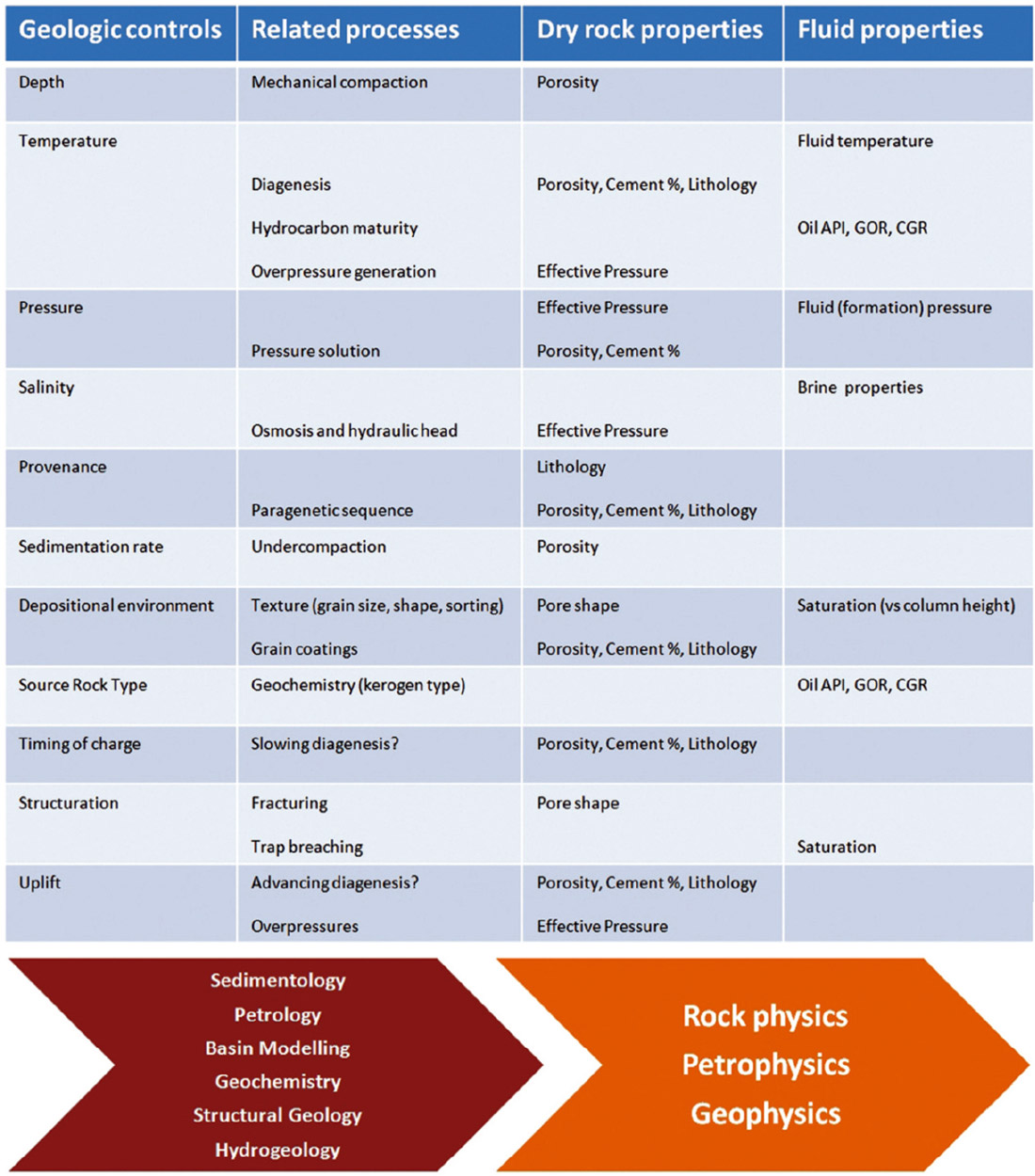
When it comes to derisking frontier wildcats, I recommend using a modification of the Gassmann equations to help structure your thinking around the geologic controls on measured seismic amplitudes, AVO and inversion attributes. Figure 8 provides a summary of the examples discussed above by linking the geologic controls and processes to their dependent rock and fluid properties.

Not all of these controls will vary laterally between calibration wells and your prospect. After consulting with a friendly and well-rounded geologist you might find that some can be safely inferred. With a bit of luck, there might remain sufficiently few unknown controls to allow quantitative predictions to be made using established AVO modelling or inversion techniques. If not, then a scenario approach to risking using seismic amplitudes is strongly suggested.