Geomechanics: Bridging the Gap from Geophysics to Engineering in Unconventional Reservoirs

Introduction

Oilfield Geomechanics has a broad range of definitions, and depending on who you ask you may get a different answer. To this author, in its simplest form, it encompasses the study of how stresses and strains within the earth affect what we drill into and explore for. The magnitude and direction of stresses and how they affect the rock properties in a region, a field, and a wellbore has a massive impact and control on what we do in unconventional resource exploration and exploitation. Unconventional in this case refers to tight sands and shales containing oil or gas that require stimulation to produce at economic rates. This paper will describe how geomechanics influences wellbore stability, reservoir properties, and hydraulic stimulations. Through this description of geomechanics I hope to convince geophysicists that there is not so large a gap between the engineers we deal with and the seismic data we look at every day.

Geomechanics basics:

Applied geomechanics deals with the measurement and estimation of stresses within the earth, and how those stresses apply to oilfield operations. Throughout this paper we will be discussing stresses within the earth, and for convenience we will use the principal stress notation where the overburden or vertical stress is denoted σv, the maximum horizontal stress as σH, and the minimum horizontal stress as σh. Stress is a force per unit area, and if we visualize a point within the earth as a cube it can be visualized as in Figure 1. This consists of three normal stresses and six shear stresses. A simple rotation can be applied to this tensor which results in the shear stresses going to zero leaving only the principal stresses shown in Figure 2. This assumes that the overburden is vertical and horizontal stresses are normal to the vertical stress (Anderson, 1951). This assumption holds true in most areas, except near large geologic structures such as faults, salt domes, and igneous intrusions where more complicated stress models are needed to describe the stresses within the earth.

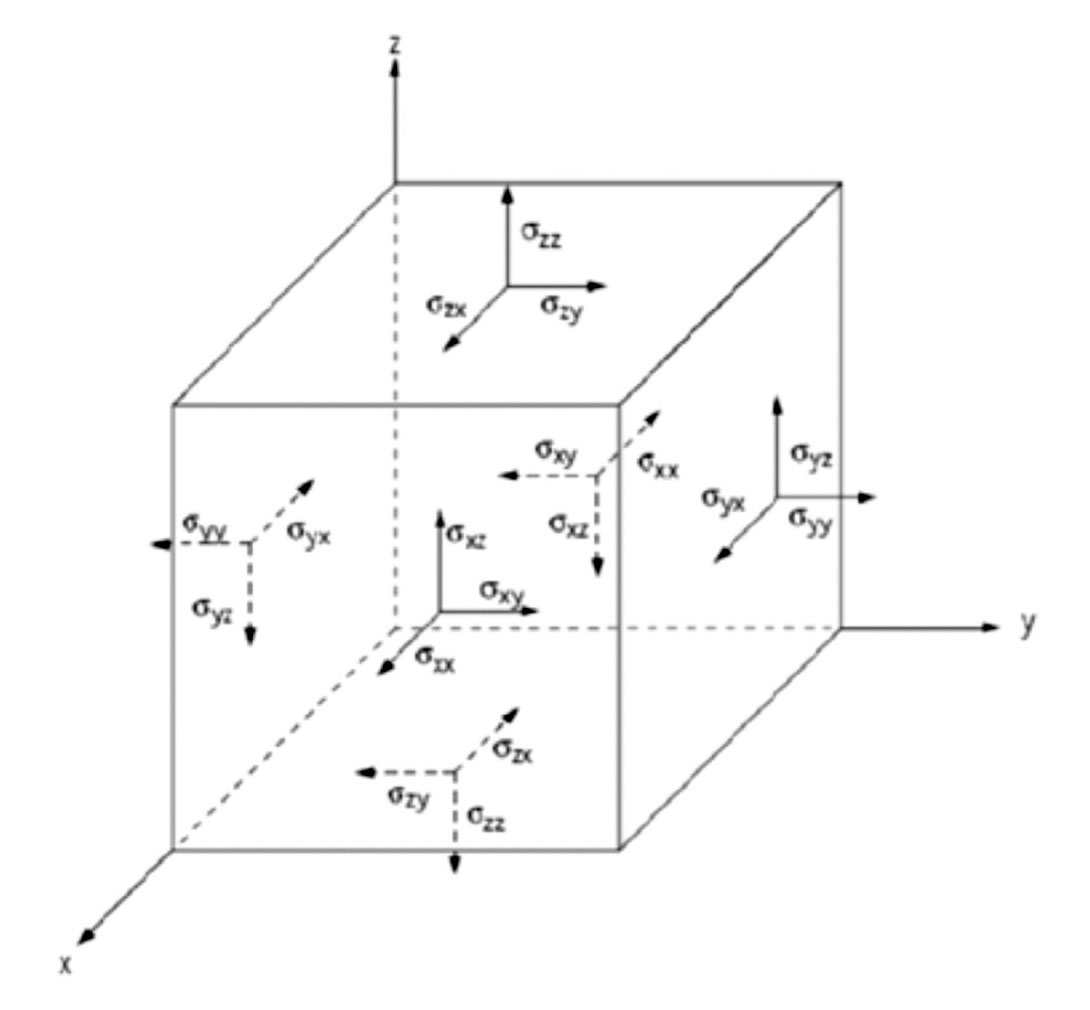
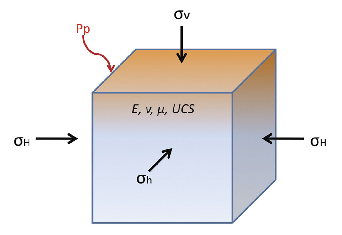
When we look at the simplified result of this diagram (rotated so no shear stresses exist), we see that we are left with the weight of the overlying rock (the overburden) and two horizontal stresses as shown in Figure 2. Now that we have defined stresses, we can get into the explanation of effective stresses. Within the earth, a formation’s strength and the fluids it contains dictates how stresses act and distribute within that formation. As a result, the pore pressure and rock properties of each formation need to be calculated or estimated to gain the full understanding of how stress acts within the earth. The pore pressure within a formation can help support the load that it maintains, and this needs to be taken into account when we estimate stresses. Terzaghi first described this relationship in 1943 with Equation 1 below:

Equation 1: Terzhagis equation where σ’ = Effective stress, σ = total stress, and Pp = pore pressure.

Within the oil and gas industry, rock properties are usually described in terms of Poisson’s ratio, Young’s modulus, bulk modulus, and shear modulus. These moduli are calculated from the P and S wave logs in wellbores and interestingly the dynamic moduli can also be estimated from seismic data (more on that link later). In addition to this, for wellbore stability purposes, we try to measure from core or estimate using empirical relations the Unconfined Compressive Strength (UCS). Full explanations of all of these moduli aren’t necessary in this paper, but those interested can find complete details in Mavko et al; 1999 and Jaeger and Cook, 2007.

It is not my intent to show how we can estimate all of these properties with well log and seismic data, but rather the impact that the results of this modeling, combined with or derived from seismic data, can have in the unconventional. Anyone interested in the construction of a geomechanical model will find these references of interest: Zoback et. al., 1985; Moos and Zoback, 1990; Sayers, 2010; Jaeger and Cook, 2007; Barton et al; 2009. It will be shown in the next few sections that the estimation of the direction and magnitude of these stresses along with the associated geologic rock properties provided by seismic can be extremely useful.

Stress directions and magnitudes; impact on the wellbore and completions:

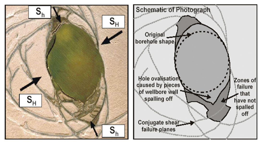
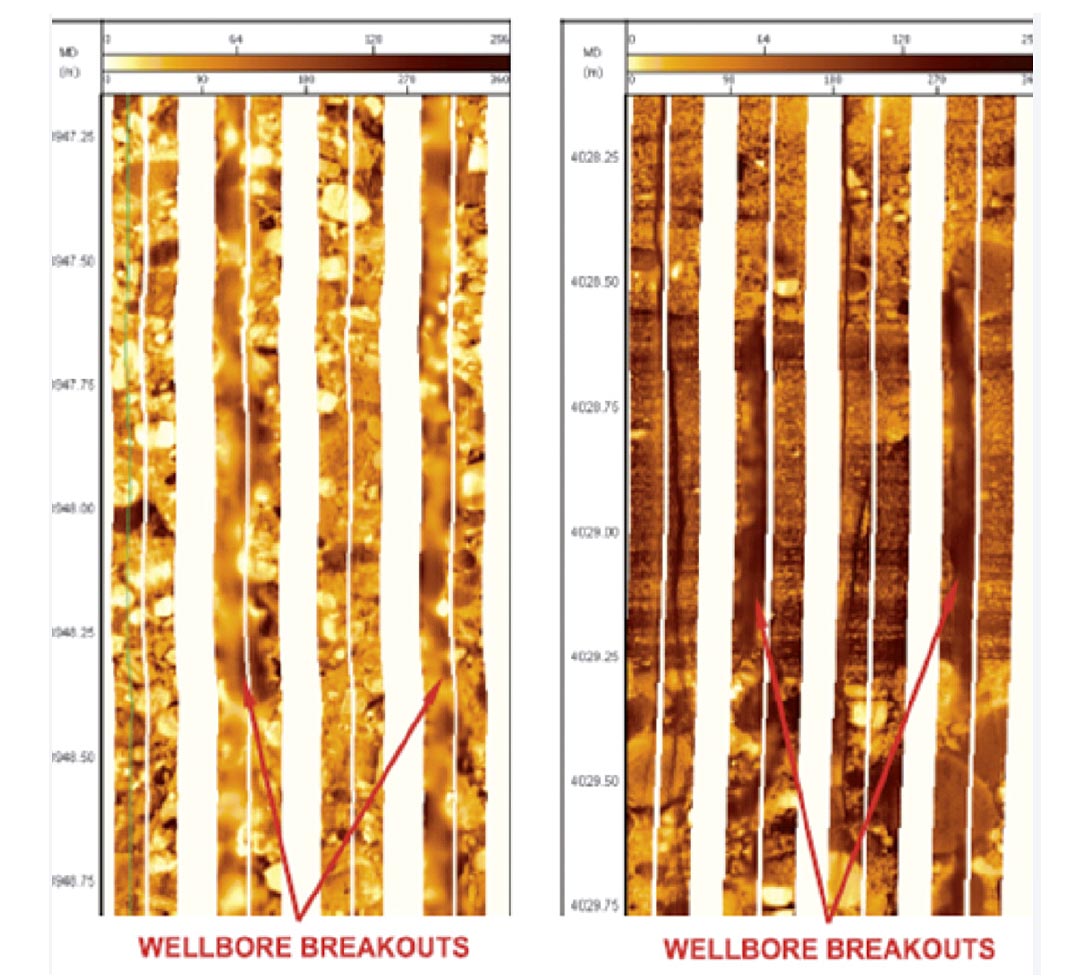
Before we put a hole in the earth, it is in a state of stress equilibrium. The borehole that we are drilling disrupts that equilibrium and causes stress to redistribute around the borehole. We have mud weight to balance this dis-equilibrium, but commonly this is not enough to stop breakout or wellbore instability completely. By looking at the damage we cause in the borehole while drilling (via drilling, tripping in or out, surging and swabbing, etc.) we can estimate the stress directions in the formations we drill through and start to constrain the magnitudes of stresses with other drilling and completion data from the area (Figure 3). If we look at an image log as shown in Figure 4, we can see that breakout has a distinct appearance (caliper logs can be used for this purpose as well). Breakouts occur in the direction of minimum horizontal stress, as the maximum compression (where breakout occurs) in the wellbore happens 90 degrees from the maximum horizontal stress (in most cases). Because of this relationship we can estimate the σH direction.

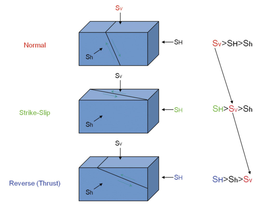
Once the directions of stress are known, it is possible to make estimates of stress magnitudes. The overburden is usually quite easy to estimate, as we almost always have density logs in the area. Simply integrating the density of the overlying rock (and water if we are in an offshore setting) and multiplying by the acceleration due to gravity will give the overburden stress. The minimum horizontal stress can be estimated using leak off tests, offset completion data, or mini fracture tests within the wellbore. The maximum horizontal stress is always one of the largest unknowns in the world of geomechanics as there is no direct way to measure it. This can be constrained either by using advanced sonic measurements (Sayers, 2010) or by using the severity of wellbore breakouts (Moos and Zoback, 1990; Barton et al; 2009). The magnitudes of the horizontal stresses are of the utmost importance as the magnitudes with depth define the type of faulting regime that the formation of interest lies in. Figure 5 shows the Anderson fault classification based on relative magnitudes of principal stresses, while Figure 6 shows data from the publically available World Stress Map (Heidbach et al; 2008).

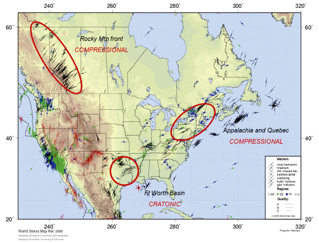
All of the information contained in this map is extremely useful for unconventional oil and gas exploration. Almost all horizontal wells completed in unconventional resource development are drilled in the direction of minimum horizontal stress. This is done to contact and prop open the largest amount of reservoir by making fractures perpendicular to the horizontal well as shown in the left of Figure 7. This also highlights how the maximum horizontal stress direction controls the direction of stimulation propagation in high horizontal stress ratio environments (strikeslip or thrust fault regime). In the left of Figure 7, which is in western Canada, the regional maximum horizontal stress direction is 45° east of north. This is also the direction in which the stimulation has grown according to the microseismic. The magnitudes of these stresses and their local variations are often overlooked, but are just as important. Take, for example, the Fort Worth Basin; which is the birthplace of North American shale gas. This basin has been used as an analogue for almost every new shale play in the past 10 years due to the large amount of publicly available data. However, the stress state in the Fort Worth Basin is one that is, for the most part, in a normal faulting regime (there are some exceptions to this); and the magnitudes of the horizontal stresses are nearly equal. Where the horizontal stress ratio is high, as in the Montney, induced fractures grow in a very linear fashion from the perforations out into the formation (left side of Figure 7 and Figure 8). In contrast, where the horizontal stress ratio is low, as in the Barnett, induced fractures are able to grow in a much more complex pattern using more of the pre-existing natural fracture network (right side of Figure 7 and Figure 9).

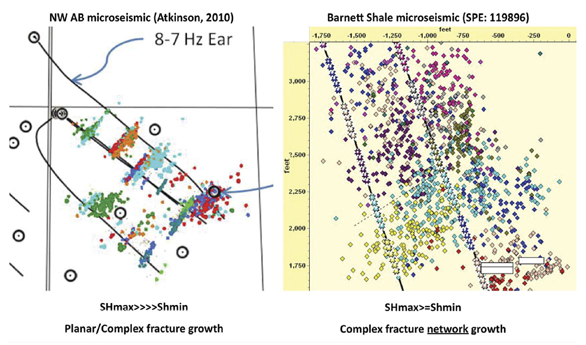
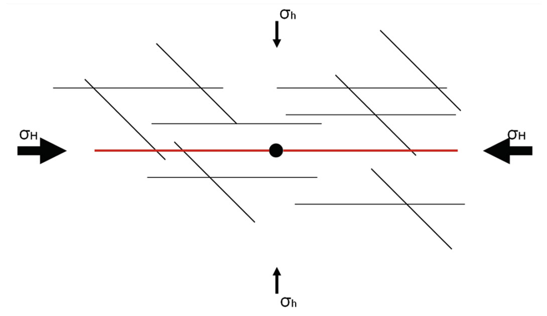
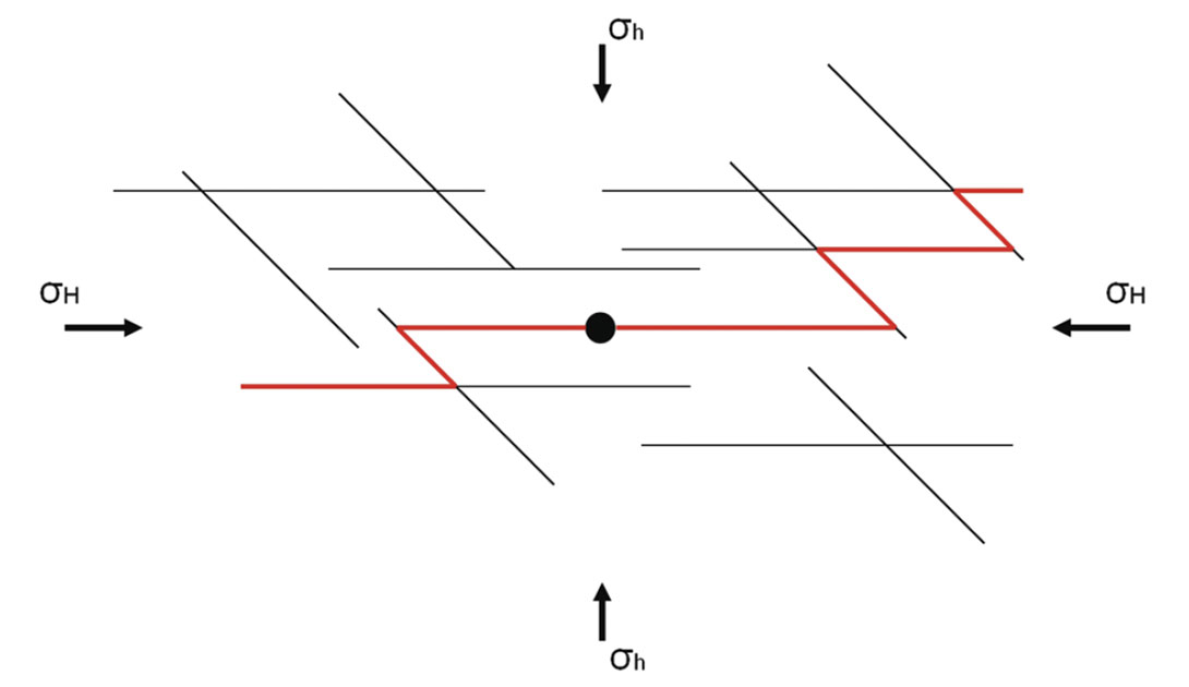
Looking at Figure 6 we can see that most other areas of emerging and abundant shale gas in North America are NOT in a normal faulting regime. Indeed, the basins that contain the Marcellus, Horn River, Bakken, Cardium, Monterey, and the Montney are almost all strike-slip or reverse, commonly with high horizontal stress ratios. Figures 7-9 all point to the fact that stress direction and magnitude matter in a way not fully appreciated by many. High horizontal stress anisotropy does not allow the growth of induced complex fracture networks that permit maximum reservoir contact. The growth of hydraulic stimulations is affected by many things outside of the completion design; pre-existing planes of weakness (fractures and especially faults), rock fabric and type, rock properties, etc. It is also important to note that while complex fracture network growth can be seen in highly compressive environments, it is usually the exception, not the rule. I will leave this topic with a quote from a paper written by King et al; 2008:

“Development of both primary and secondary fractures is possible when the maximum and minimum stresses are relatively similar. When tectonic stresses are highly dissimilar, switching fracture directions will be difficult and complex fracture development improbable.”

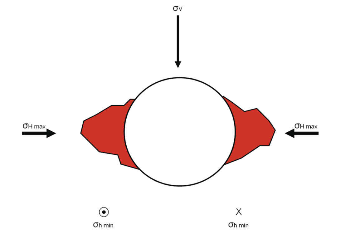
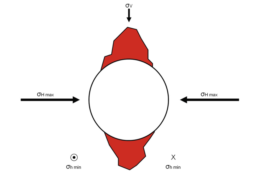
On top of the control on hydraulic stimulations, ratios of stresses within the earth control important details of how the wellbore breaks out in both the vertical and horizontal well section. This phenomenon is especially important, keeping in mind that these wells are nothing without a completion, and the cement job can greatly affect a stimulations effectiveness. In most cases people visualize breakout (or compressional failure) occurring (Figures 10 and 11) in a horizontal well on the sides of the well due to the weight of the overlying rock. This ovalization of the wellbore is problematic but easier to clean than the alternative. In highly compressive environments like strike-slip or thrust fault regimes, this breakout occurs not at the sides but at the top and bottom of the wellbore. This occurs wherever at least one of the horizontal stresses is greater than the vertical stress, i.e. in NW Alberta, NE British Columbia, and Appalachia (see Figure 6). This creates many more operational problems from stuck pipe, hole cleaning, well logging, and cement jobs.

When drilling these unconventional wells, the norm is to drill with as low a mud weight as possible to increase the rate of penetration and therefore speed up drilling and reduce the amount of rig time paid. This approach is usually not conducive to reducing breakout, because once it occurs; it tends to be self sustaining (see Figure 3). As the drill pipe is pulled out and put into the hole the pressure changes, this is known as surge and swab. When this occurs in a highly compressive environment, the potential for stuck pipe increases dramatically as rock falling from above has a much greater chance of causing tight spots and stuck pipe. If we knew that this compressive environment existed pre-drill, it would allow us to come in at a more appropriate mud weight, and therefore reduce or avoid altogether the severe breakouts that lead to serious operational setbacks.

Rock Properties:

In addition to regional stress directions and magnitudes, the properties of the formation itself are of great importance. This importance is not limited to building a complete geomechanical model; but also to assess our ability to break the rock with a hydraulic fracture, the formation’s strength when we drill through it, and how these rock properties relate to and control seismic wave propagation. I will concentrate primarily on how properties that we can derive from seismic using currently available techniques can be used for stimulation modeling and proppant selection. To move forward, a proper definition of the terms we are using is needed. This is followed by an introduction to how the rock properties as defined are used in drilling and completions engineering.

If we apply an increasing vertical load to a core plug, and leave the sides unconfined, the load will deform until it fails at the uniaxial or ‘unconfined’ compressive strength. This parameter is known as the UCS and is sometimes denoted as the rock’s “strength” by drilling and bit companies. This failure cannot be recovered (we broke the rock) and is therefore inelastic. The remainder of the terms that we are dealing with will be in the realm of the elastic, i.e. the loads that we apply are theoretically recoverable and do not go into the realm of plastic (or unrecoverable) deformation. More background on this can be found in Jaeger and Cook, 2007. The definitions below, summarized in Figure 12, are from Batzle et al; 2006.

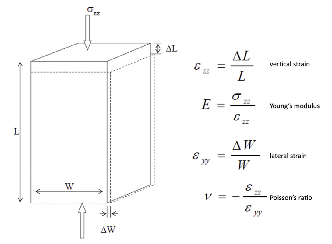
For an isotropic and homogenous medium, we apply a vertical deformation (ΔL) associated with the vertical stress. Normalizing this deformation by the original length of the sample, L, gives the vertical strain ε_zz. By definition, Young’s modulus, E, is the ratio of applied stress (σ_zz) to this strain. Young’s modulus is therefore in units of stress (MPa, psi, etc.). This same stress will generally result in a lateral or horizontal deformation, ΔW. The lateral strain is then defined like the vertical strain and is denoted ε_yy. The relationship of these strains (vertical to horizontal) is known as Poisson’s ratio. The negative sign is attached because the signs of the deformations are opposite (vertical negative, horizontal positive).

In the oilfield, these rock properties can be derived from the P and S waves of modern sonic tools. Properties derived from logs (and seismic) are known as dynamic moduli, meaning that they are measured with sonic waves and need to be calibrated to laboratory measurements (static). There is much debate about the validity and the problems of up-scaling when moving from core scale, to logs, and then to seismic. This is because we tend to sample cores that are competent and un-fractured; and also because of the dispersion that occurs due to the different lengths of measurements used to measure these dissimilar scales. We know that in almost all cases fractures play a part at some scale and that dispersion due to measurement length always affects our accuracy. These issues aside, in the oilfield Young’s modulus (E) and Poisson’s ratio (ν) have become ubiquitous in both geomechanics and in engineering. Because of this they should also become common place in the geoscience world.

In hydraulic stimulation modeling, E is used as a proxy for how wide a crack can be opened in a formation, and is therefore used to pick perforation locations in both vertical wells, and when available, horizontal wells. A lower E means that a wider crack can be opened and therefore flow increased during the stimulation and more or sometimes larger proppant used. Since we make almost all of the permeability we will ever have in tight sand or shale oil and gas, this is an important parameter. At depths where the overburden is not the least stress, the minimum horizontal stress can be calculated using the uniaxial strain equation (Equation 2). This equation assumes that the reservoir is linear, homogenous, and that there is no tectonic strain caused by the tectonic component of stress (Hubbert and Willis, 1956 and Teufel, 1996). In most situations, tectonic stress and the resulting strains will be appreciable. Most stimulation simulators use modifications of this equation to account for tectonic effects, but these are in most cases poorly constrained and often just calibrations to existing stress data (minifracture tests, leak off tests, etc.)(Blanton and Olsen, 1999).

Equation 2: Uniaxial elastic strain model where σ_h = minimum horizontal stress, σ_v = overburden, ν = Poisson’s ratio, α = Biots constant, and Pp = pore pressure.

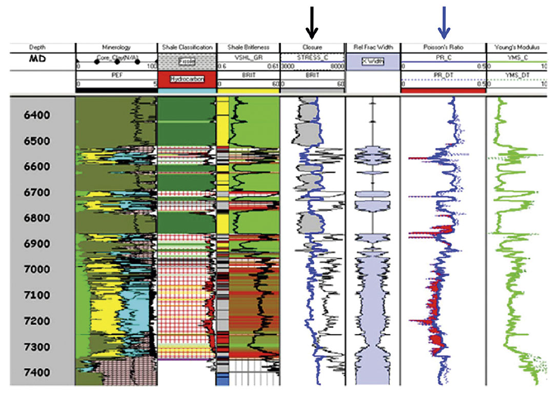
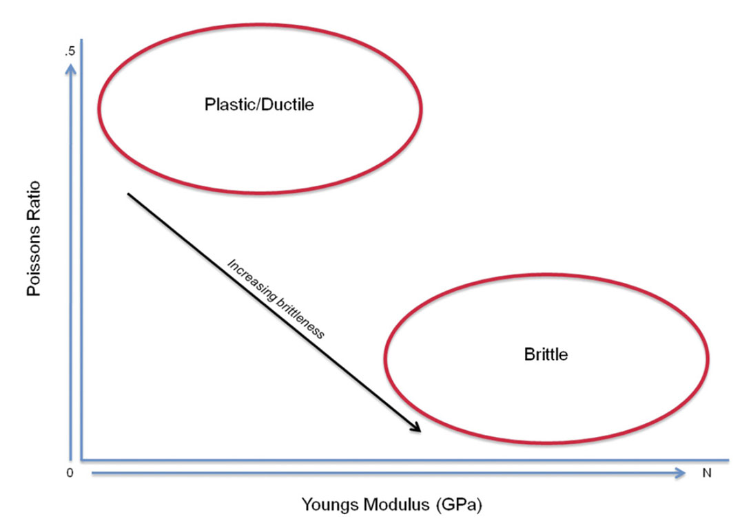
In addition to the importance of E and ν for stimulation modeling, petrophysicists have recently begun using these two well log derived rock properties as a proxy for rock ‘brittleness’ or ‘ductility’ (Rickman et al; 2008). A rock’s brittleness or ductility is influenced by many parameters outside of E and ν: the grain size and distribution within the rock, mineralogical content, and especially the fracturing of the formation all influence how easily a rock will break during stimulation. It is no secret though that our ability and time to measure these things are always limited, especially in the unconventional where turnaround from logging to completion varies from days to weeks. This usually doesn’t allow for in-depth lab testing to be performed. We are left then using E and ν for local and regional estimations of a formation’s brittleness, hopefully calibrated in some way to regional core measurements. This allows us to have an idea of the formation’s mechanical properties prior to perforating and stimulating. This concept, from Rickman et al; 2008, is shown in Figure 14.

Seismic rock properties and stress estimation:

The use of rock property estimation coupled with an estimate of the natural fracture density, either from AVO methods or seismic attributes, has become the method of choice for geophysicists searching for ‘sweet spots’ in shale basins (Goodway et al; 2006 and Changan et al; 2009). It has only been recognized recently, however, that we can use conventional P-wave (making certain assumptions) and multi-component seismic (Cary et al; 2010) to gain estimates of the horizontal stress directions or their ratios in the subsurface. In essence, if we have dynamic estimates of the E, ν, horizontal stress ratios, and accurate formation velocities, we have an initial estimate of the geomechanical model before the first horizontal wells are drilled.

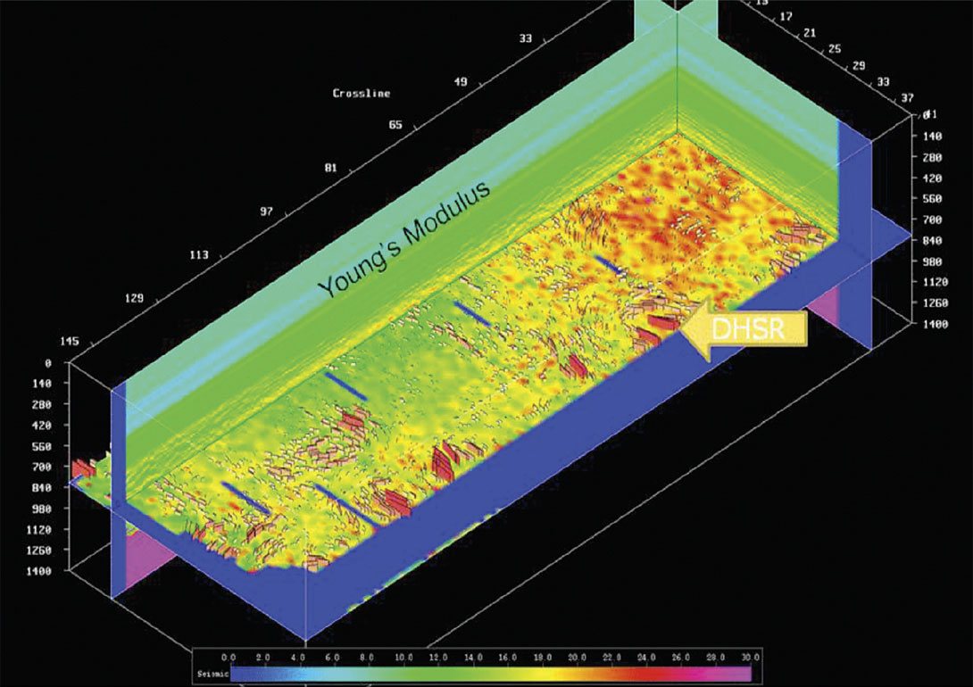
Gray et al; 2010 outlined just how this can be done using conventional P-wave seismic and AVO lamda/mu/rho (LMR) analysis coupled with assumptions to ascertain horizontal stress ratios. The method outlined by Gray allows for the estimation of differential horizontal stress ratios (Figure 15) and dynamic rock properties from 3D P-wave seismic within one 3D seismic volume. Given what we know about unconventional geomechanics discussed above, this information away from the wellbore allows for much more advanced analysis pre-drill.

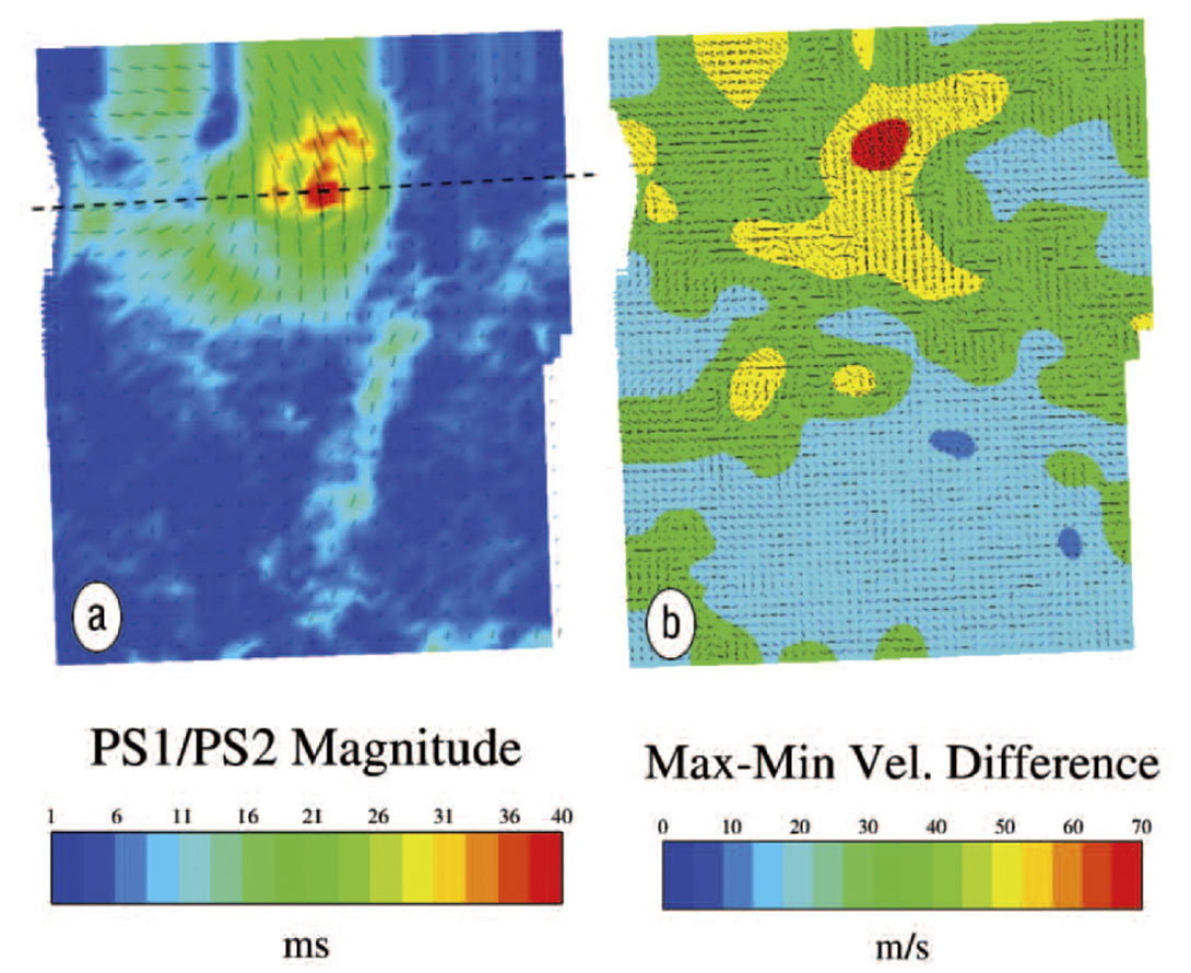
In addition to this Cary et. al. have recently shown that the difference in converted wave fast and slow velocities in the near surface can be indicative of differences in horizontal stresses as they deviate from the regional stress (Figure 16). Shear wave splitting is usually attributed to vertical cracks or fractures in the subsurface at depth. However, this splitting is observed in compliant rocks in the near surface where fracturing is known to be extremely minimal from regional core observations. Most of the fast shear (S1) direction is in the regional direction of maximum horizontal stress as derived from the World Stress Map (Heidbach et al; 2008).

We now have the ability to ascertain fracturing or stress state in a reservoir pre-drill, this is in addition to our ability to derive rock properties from conventional AVO or AVAz. Given what has been outlined in this paper, it is evident that P-wave and multi-component seismic can provide insights into geomechanics and engineering problems that are abundant in unconventional resource exploration. A 3D seismic survey (either P-wave or multi-component) can give initial estimates of fracturing or stress state, this can be further constrained when combined with local well data if it is available. In addition to this, estimates of the dynamic Young’s modulus, Poisson’s ratio, and density are possible if the data has adequate offset and azimuth coverage. When we combine this with regional well data of drilling events, logs, and completions we are well on our way to a geomechanical model before the first horizontal wells are drilled.

Conclusions

Geomechanics is not just an important parameter in analyzing an unconventional reservoir; it is perhaps the most important control on how our tight/shale reservoirs are developed. It dictates how our wellbores breakout and fail, the direction and areal extent of our hydraulic stimulations, the size and strength of proppant, how much that proppant could embed over time with pore pressure depletion, and a reservoirs mechanical characterization. Engineers use these parameters in their calculations and modeling, but ultimately the quantification of regional stresses and rock properties comes from geoscience data. Unconventional resource plays demand integration across teams and geomechanics bridges the gap from geology and geophysics to engineering in a way that is only now becoming more widely appreciated. Seismic surveys contain a large amount of data that can be utilized for geomechanical and engineering purposes before the first pads are ever drilled. All we have to do is use them.

Acknowledgements

This work would not have been possible without the help of Tom Bratton, Tom Davis, and Shannon Higgins who initially started me down the path of seismic and geomechanics. In addition, John Logel, Eric Andersen, Geoff Rait, Dave Gray, Jared Atkinson, and Rob Kendall have all provided help and insight into these issues over the past 2 years.