Geophysical Constraints in Geostatistical Modelling

Abstract

This case study, focused on a Cretaceous aged Mannville Group pool under water flood, illustrates the benefits of utilizing a quantitative and deterministic geomodelling workflow for reservoir characterization. Geophysical, geological and petrophysical data are integrated into a deterministic static model for simulation. The results of the simulation, in conjunction with pressure transient analysis and material balance calculations, have been used to alter the water injection pattern. The altered water injection has halted the production decline and led to improved recovery with no capital spending.

1. Introduction

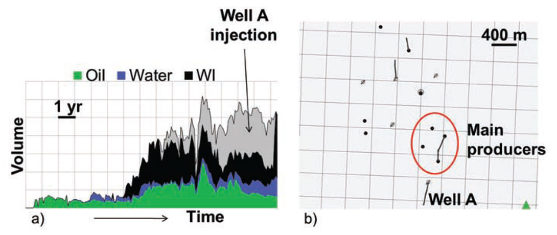
The underperforming oil pool, ‘Pool M1’, has nine active producers of which four account for over 75% of the production, and three active injectors (Figure 1). Injection has been concentrated in Well A (Figure 1) in recent years, under the expectation that as the most proximal injector to the best producers it would be the best site for increased injection volumes. Despite being on water support for a number of years, however, reservoir pressure in the Pool has continued to decline and development activity has been stymied by a lack of understanding of reservoir connectivity and continuity.

The reservoir geometry is complex and variably continuous due to the dynamic, near shore depositional environment in the area at the time of deposition. There is evidence in core, log and seismic data of shallow marine deposition, barrier island development, storm events, and fluvial/estuarine channels in the area. The interaction of these environments results in stacked reservoir quality sands that pinch out laterally, due to both non-deposition on paleo-highs or erosion and removal, and shale barriers and baffles that are difficult to map.

Despite injection volumes exceeding produced volumes for several years (i.e. a voidage replacement ratio >1 for approximately one-third of the duration of the water-flood) the reservoir pressure remained in decline. Based on the geological maps (created primarily from log data) used to plan the water-injection pattern, there was no indication that the primary injection well was not connected to the main reservoir. The reservoir characterization and simulation study presented herein was initiated to improve understanding of the reservoir and to provide recommendations regarding flood optimization and infill drilling.

2. Geomodelling

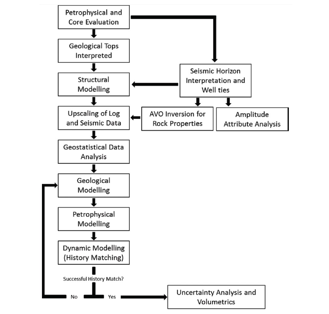
Workflow A relatively standard framework and geostatistical modelling workflow was applied in this project (Figure 2), with the aim of creating a realistic reservoir property model (or models) incorporating all available data. Data types included in geomodels can be categorised in a number of ways:

1. Deterministic and inviolable: such as well log data (‘hard data’) and Pressure-Volume-Temperature (PVT) data from core measurements (although in reality there is of course uncertainty and error in log measurements and core studies it is not typically an aim of geomodelling to assess this type of uncertainty).
2. Deterministic but with uncertainty that may be addressed systematically: such as depth converted seismic horizons and fault connectivity interpreted from seismic data.
3. Conceptual or experiential information: such as results from offset and/or analogue fields, information from outcrop studies and surface mapping, and understanding of depositional environment from regional studies.
4. Statistical information: such as variograms based on log and/or seismic data covariance as a function of distance, histograms of data distribution, and measures of correlation based on regression analysis.

A key excursion, in this field study, from a typical geomodelling workflow, was the methodology of geological modelling. In the geological modelling step geostatistical gridding or interpolation techniques, which are commonly employed, were rejected in favour of a manually constructed model. The rejection of geostatistical methods for geological modelling was necessary to ensure that key boundaries, inferred from seismic interpretation, were captured in the geological model.

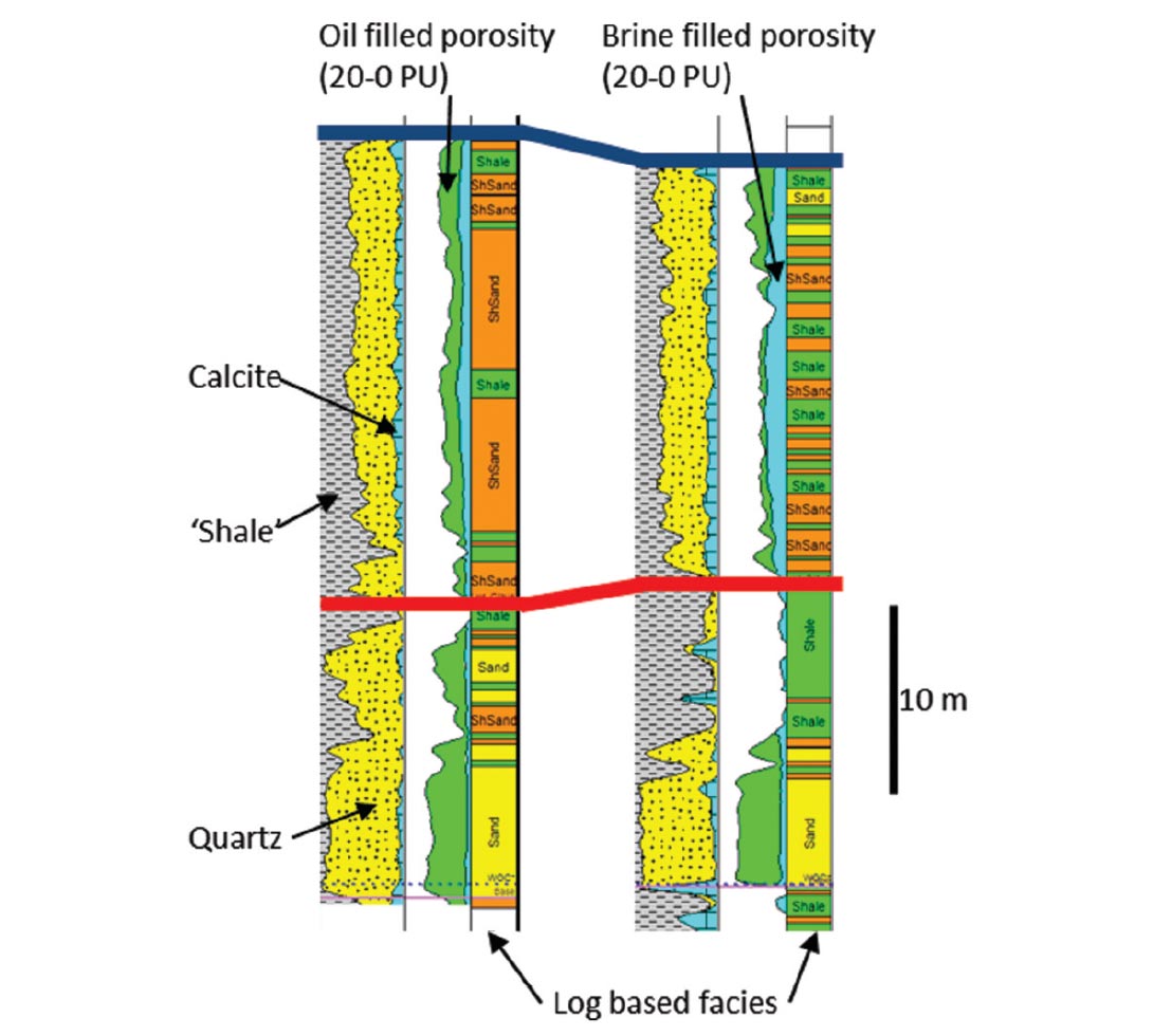
To prepare the available log data, detailed petrophysical analyses were completed on all wells within the field. Core data from three wells were used to calibrate the petrophysical processing and constrain the bounds of porosity and relative mineralogical abundance estimates. Reservoir quality sands typically comprise over 90% relatively well sorted quartz sand, with porosities that range from 8-18%. The processed log data were used to create a relatively simple facies log, based on porosity and lithology, comprising sand, shaley-sand and shale; where only the latter is considered non-reservoir (Figure 3).

The structural framework for the reservoir model of Pool M1 is relatively simply defined due to a lack of faulting. A bounding upper surface was defined using a depth-converted seismic horizon, appropriately tied to well data, and available geological tops. The base of the reservoir is difficult to define seismically and was defined from geological tops only. Due to the conformity of the bounding layers and the relatively consistent isopach, model creation is largely insensitive to layering technique. A proportional layering scheme was employed, with an average layer thickness of approximately 1 m. The limited extent of the field results in a total of fewer than 400,000 cells using a 50×50 m grid, this is a feasible quantity for simulation. The number of cells in a model is a critical consideration for all static models intended for dynamic modelling due to the computational expense of simulation with very large numbers of cells and the necessity of running multiple simulations in almost all dynamic modelling studies.

Conditioned and processed log data were upscaled to the geocellular model using standard techniques for continuous properties (e.g. arithmetic mean for porosity, acoustic impedance, etc.) and discrete logs (e.g. ‘most common’ or ‘most of’ for facies or rock type). Water saturation and permeability log estimates were not upscaled, however, as it is preferred to define these properties on the basis of rock type and core-based Pressure-Volume- Temperature (PVT) measurements after the model is populated appropriately.

3. Geophysical Inputs and Data Preparation

3D seismic reflection data covering Pool M1 were re-processed using an AVO compliant flow that included 5D interpolation and pre-stack time migration, to improve imaging and prepare the data optimally for AVO inversion. Following careful well ties, including analysis with both zero-offset and non-zero-offset synthetics, critical horizons were interpreted on migrated stack data to assist in the interpretation of reservoir structure and geometry.

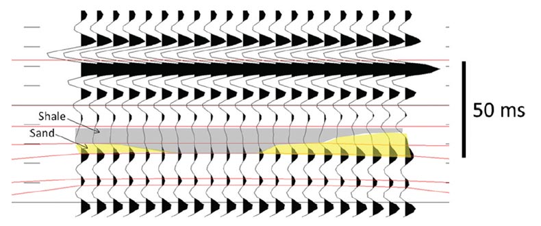
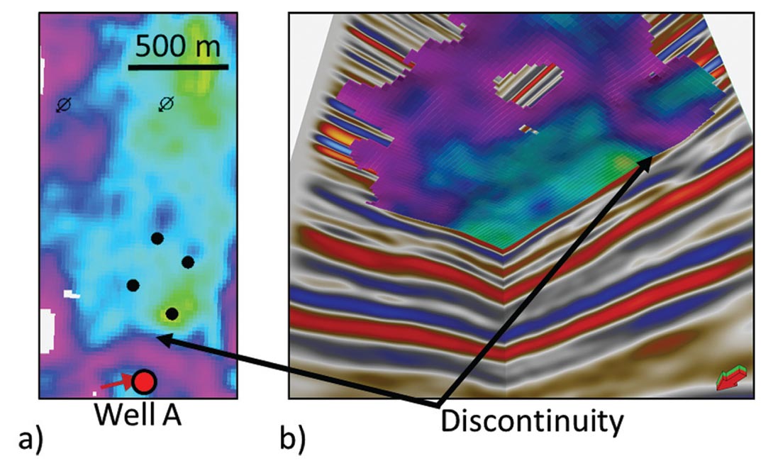
Simple zero-offset synthetic modelling, based on well log data, illustrates the predicted impact on the seismic reflection of changing the ratio of shale and sand within the reservoir (Figure 4). Increased sand thickness corresponds to an increase in the trough and peak amplitude at the top and base of the reservoir respectively. The higher impedance of the underlying clastic package results in a greater relative increase in the peak amplitude at the base of the reservoir, relative to the trough associated with the top of the reservoir. Accordingly, amplitude extractions and full stack attributes (such as RMS amplitude and sum of positive amplitudes) extracted over the zone of interest correlate strongly to petrophysical maps of reservoir thickness and quality. Such attribute maps also assist in imaging potential reservoir boundaries, as illustrated in Figure 5. An obvious change in amplitude character is captured in the map in Figure 5, which can be seen to correlate to an extreme thinning in the positive peak at the base of the reservoir that is interpreted to represent either non-deposition in the region of a subtle paleo-high or erosion of reservoir sands. Although insights from the full stack amplitude data are of great utility in terms of reservoir characterization, there is potentially much greater uplift from AVO inversion of the amplitude data.

Estimates of rock properties based on AVO inversion can provide important constraints on property distribution in geomodelling workflows. Relative to well log data, the dense lateral sampling of seismic reflection and inversion data (30×30 m bins in this survey) provides substantially higher spatial frequency. If either full stack seismic amplitudes or rock properties estimated from AVO inversion can be positively correlated to reservoir properties of interest, such as lithology or porosity, their inclusion in the geocellular model can significantly decrease the uncertainty in property distribution (where uncertainty is defined in this instance as the range of potential solutions for a given cell within the model).

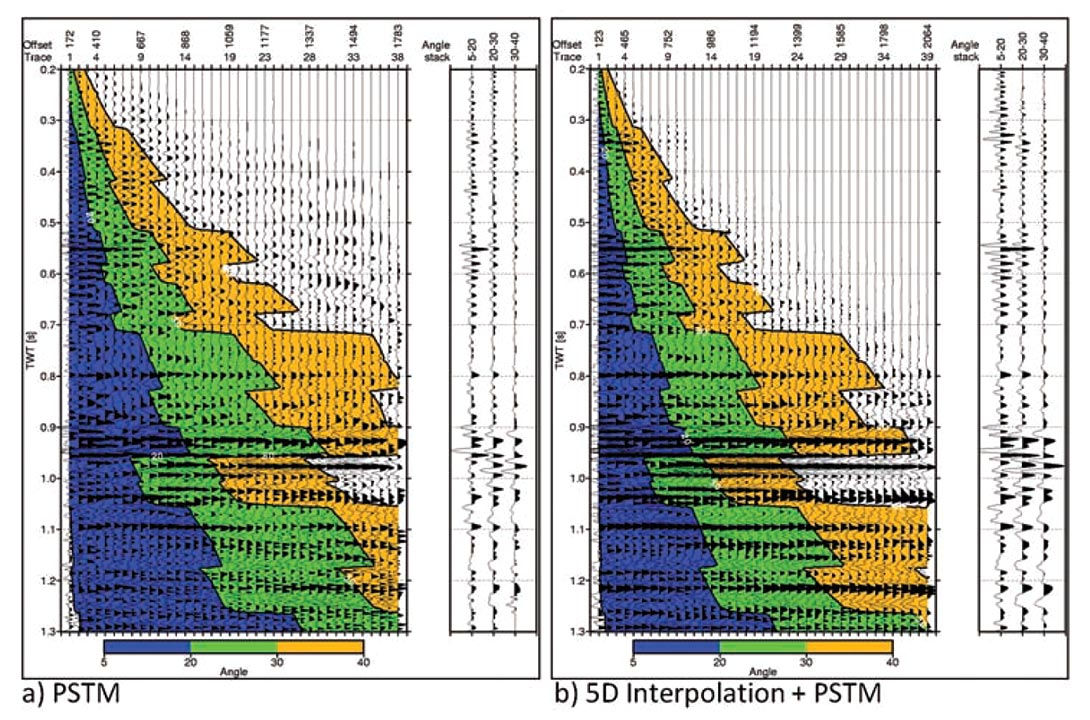
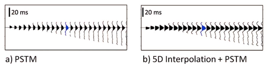
AVO inversion testing was completed on PSTM data with and without 5D interpolation having been applied (Figure 6). The lateral continuity of reflectors is clearly improved by the interpolation process, as is the overall signal-noise ratio. However, after stacking angle-limited traces to form angle stacks the difference is, predictably, less marked (Figure 6). As the power of stacking multiple traces into the angle stacks reduces the visible impact on the gathers it also reduces impacts on wavelet extraction that might be expected based on gather analysis (Figure 6). Wavelets extracted from the near angle stack, using log data, with and without 5D interpolation have a similar appearance in the time and frequency domain (Figure 7). Inversion results are very similar for the non-interpolated and 5D interpolated data – the limited population of shear log data from the field prevents a quantitative assessment of the uplift, if any exists, of using 5D interpolated data in AVO inversion.

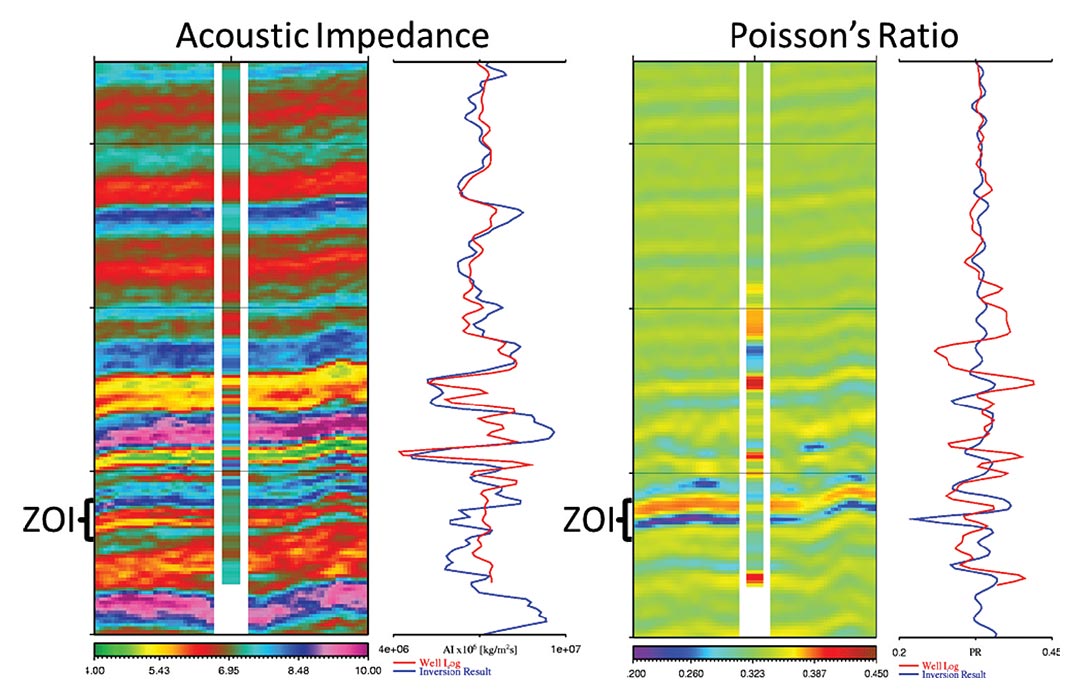
Model based inversion for Acoustic Impedance (AI) was relatively successful, as illustrated in Figure 8 where the major AI anomalies are predicted by the inversion result (the low-frequency-model was very simply defined and is close to a constant value throughout the inverted section). Attempts to accurately predict Poisson’s Ratio from the inversion were less reliable (where testing was possible; Figure 8). Significant effort was expended to improve the AVO inversion, including testing multiple deterministic and statistical wavelets extracted over different windows (including and excluding the overlying coals) and inversion methodologies, however, the results remained largely unchanged. Due to the uncertainty in the accuracy of the shear velocity based inversion results, which is difficult to assess quantitatively with limited shear log control, the AVO inversion outputs could not be used in isolation to confidently predict lithological variation across Pool M1. Seismic amplitude data in conjunction with the AVO inversion volumes, however, can be correlated to estimates of reservoir quality based on gamma-ray, neutrondensity and sonic logs.

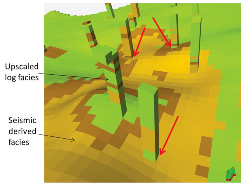
Given the qualitative positive correlation between seismic amplitudes and acoustic impedance, inversion and seismic amplitude data were used to define geobodies representative of lithology within the reservoir. These geobodies were upscaled to the geocellular model, creating a ‘geoseismic’ model of the reservoir. The relatively coarse lithological units defined in the geoseismic model were further refined using the upscaled facies logs based on well data. It is clearly necessary that a consistent facies or geological model is defined, and any misfit in lithological prediction between well log and seismic geobody definition must be reconciled. As the log data are considered hard data, the geoseismic model was manually adjusted to honour the well log based facies and thus construct a fully populated geological or facies model.

4. Geomodelling

Despite the relatively good correlation between seismic predicted reservoir and log measured reservoir intervals, a substantial amount of detailed editing was required (Figure 9). Editing such as this cannot be automated easily and is based on a geologist’s understanding of the depositional environment and interpretation of log data continuity. Although manual construction of geological models within geomodelling software is relatively time-consuming and subjective, it remains necessary that knowledge regarding the geology of a reservoir is captured in such a model. In utilizing purely geostatistical techniques and log data it is inevitable that knowledge and experience is not optimally captured in a model in many cases. Although through the coupling of geostatistical techniques and multipile stochastic realizations it is possible to assess uncertainty in volumetrics and property distribution, this is not always the focus of a study. This is a critical point to understand in all geomodelling studies.

Probabilistic or stochastic techniques for creating a geological model were tested, but deemed unsatisfactory due to the inability of such techniques to honour the boundaries inferred from seismic interpretation (even using trend maps and seismic constraints). The deterministic and manually edited geological model derived from the well log data and the geoseismic model enabled the petrophysical properties modelled to honour individual distributions observed for each facies. This brings significant uplift in terms of the level of detail that can be utilized in defining property distributions (Figure 10).

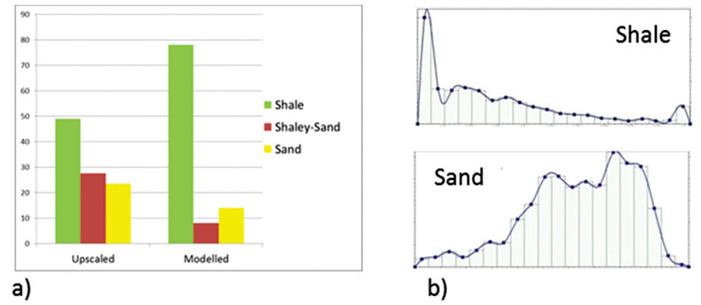
Additionally, one ‘rule of thumb’ that can be elegantly avoided by taking a deterministic approach to geological modelling is that the well log distribution of any given property should be honoured in the final property distribution. This rule or guideline is based on the notion that what is observed in the wells should be honoured on a larger scale, but this makes an implicit assumption that the well data are representative. Rarely is it the case, however, that wells are truly representative of the geology on the scale of a full-field model, the wells have likely been drilled intentionally to intersect hydrocarbon bearing reservoir. Accordingly, our statistical distribution from well log data is biased.

Figure 10 illustrates the proportion of the three modelled facies after upscaling and after distribution throughout the geocellular model, clearly in the model for Pool M1 there is substantially lower proportion of reservoir rock in the final model than in the wells. If this were not the case, and the original proportions were honoured, volumetric estimates of oil and/or gas would be overestimated. Indeed, when stochastic distribution techniques are employed and original distributions honoured there are typically prospective reservoir zones emplaced haphazardly away from well control that have no basis in reality but are required to maintain the property proportions even outside the reservoir limits, this can create obvious problems for inexperienced geomodellers.

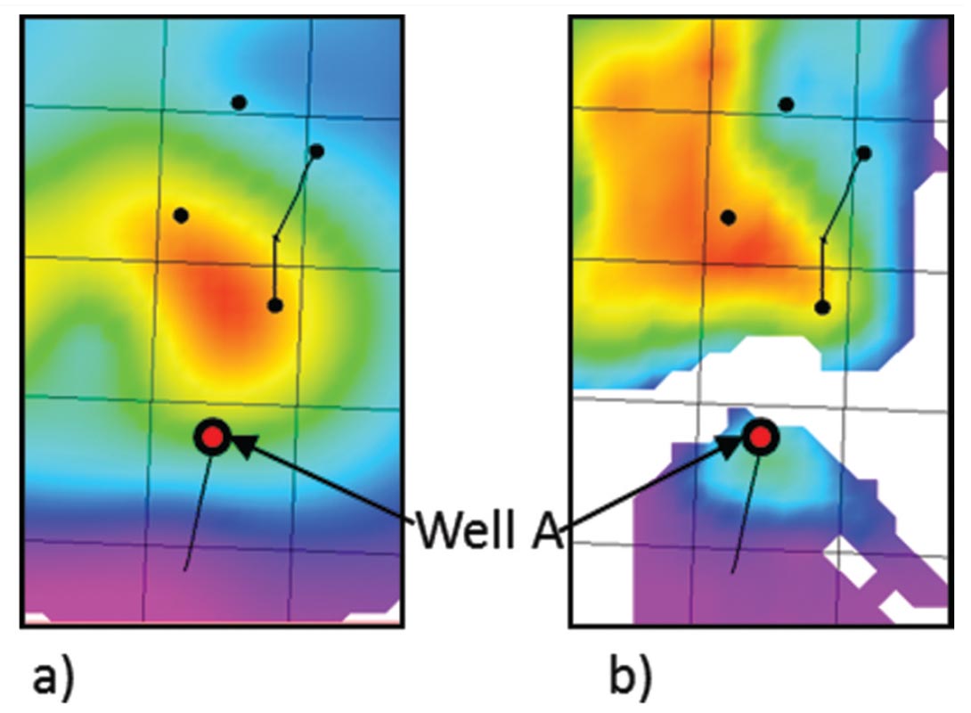
Utilizing distributions of petrophysical properties defined for each facies with a single deterministic facies model it is possible to generate multiple ‘constrained stochastic’ realizations of petrophysical properties. The primary difference of relevance between the deterministic model constructed and all stochastic distributions is the lateral facies change between the primary water injector and the cluster of main producers indicated in the seismic attributes; such a boundary cannot be inferred from log data alone (Figure 11). Whether the final property or static models are an accurate representation requires independent verification, in this case dynamic modelling was undertaken to establish the accuracy of the model.

4. Reservoir Simulation

The first-pass static model for Pool M1 was passed to a simulation engineer for dynamic modelling. The layering and cell dimensions had been chosen such that no further upscaling was required before simulation. We consider that it is optimal, where possible, to create the geological model at the resolution appropriate for simulation.

Initial simulations were successful in matching the field wide production through time. However, at individual wells there were instances where water breakthrough occurred too rapidly, indicating that a baffle in the reservoir had not been captured in the model, and also where the gas-oil ratio was too low in the model relative to the observed history. Areas such as these, where anomalies in the history match occurred at individual wells, were examined in closer detail and changes to the static model made.

The feedback loop, between geoscientist and engineer, is critical in establishing an accurate geological model and is preferred to the reservoir engineer simply making any alteration necessary to the model to match the field-wide and well-by-well production histories. In all instances where the initial static model failed to history match individual wells there was increased uncertainty in the original model due to a lack of data or the original exclusion of data (due to uncertainty in the deviation of a single well in one case), which allowed adjustment of the static model without violating any observed data or sound geomodelling principles.

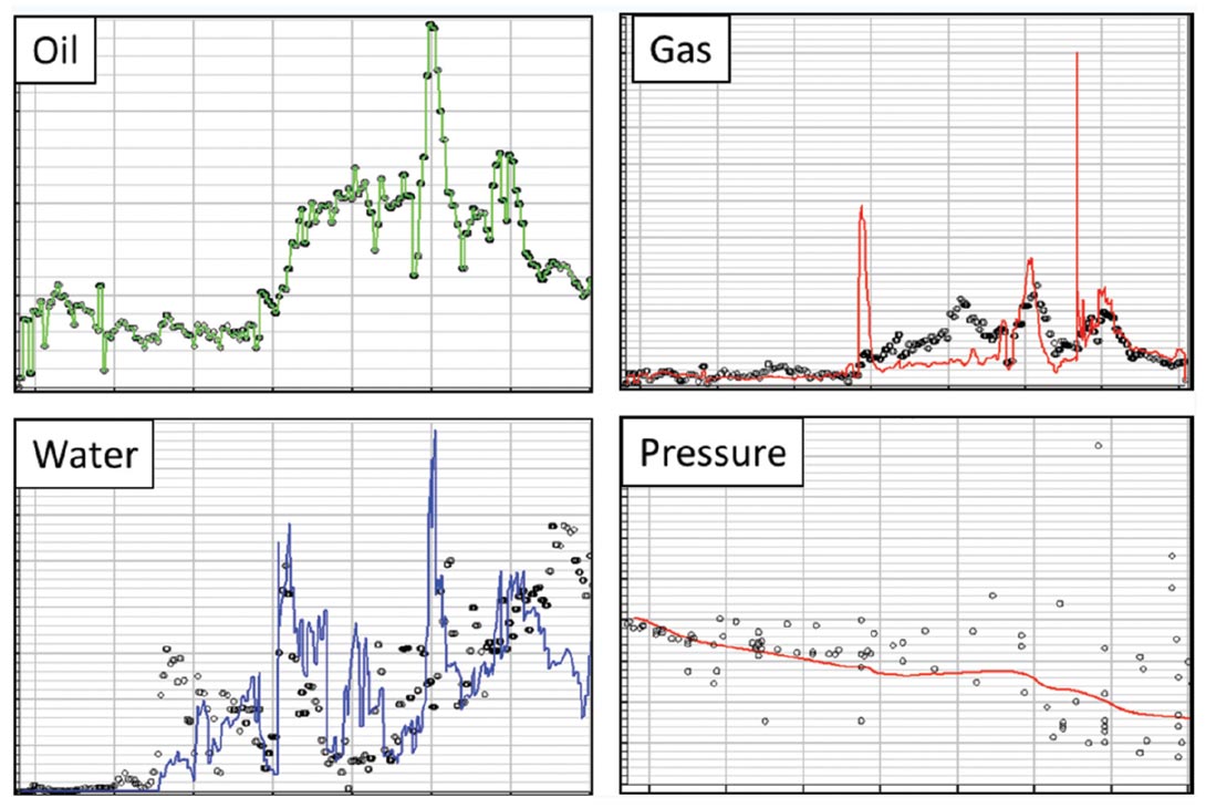
The successful history match illustrated in Figure 12, achieved after several iterations between static and dynamic modelling, provides confidence in the accuracy of the geological model to mimic fluid flow within the field. The primary conclusion drawn from the reservoir modelling was the confirmation of a discontinuity in the reservoir that was interpreted in seismic amplitude and attribute data. This discontinuity is of critical importance as it is located between the primary water injector (Well A) and the producing wells. This explains why, despite the cumulative voidage replacement ratio being greater than 1, the pressure within the reservoir continued to decline. Injection to the nonconnected well was ceased and all injection volume diverted to two within unit injectors with sufficient capacity to handle increased injection.

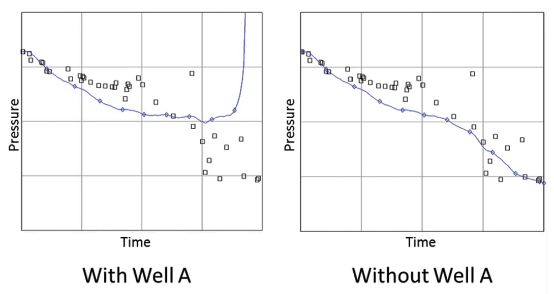
Independently of the geomodelling study a simple material balance study was completed and Pressure-Transient-Analysis (PTA) undertaken on Well A. The results of the material balance study (Figure 13) provide further evidence that Well A is not connected to the main reservoir. In Figure 13a it is evident that if the volume of water injected into Well A was in communication with the reservoir then pressures would be far above virgin, which they clearly are not. When volumes injected at Well A are excluded there is a very good match between modelled and observed pressures. This example shows the obvious benefit of material balance studies in fields under secondary recovery. The PTA results also indicate that Well A is affected by a boundary, which is interpreted to be associated with the reservoir boundary interpreted from 3D seismic data. These results in conjunction with the geomodelling study provided powerful evidence to support a drastic change in the water flood and abandon injection in Well A.

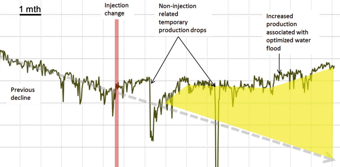
Subsequent to iterating through cycles of geological model adjustments and history matching, field production was forecast through 30 years to assess sweep efficiency. Forecasts were completed with the present day configuration of producers and injectors (excluding Well A), and also with various combinations of added producers and injectors to select an optimal number of infill wells to maximize reserves with an acceptable amount of production acceleration. The status quo forecast (i.e. with no additional drilling) indicates that the change in injection alone would arrest the decline in oil production and result in increasing production for 2-4 years. Production data support this forecast (Figure 14) and illustrate that production has increased, as water cut has dropped, without any further drilling. This production result, which is undeniably a result of the change in water flood configuration, is further validation of the accuracy of the static model created.

5. Conclusions

Geophysical, geological and petrophysical data were integrated into a static model that under simulation successfully history matched historic production. Key to the success of the model was the utilization of seismic data to provide a qualitative reservoir geometry that was then tied manually to well-based facies descriptions. The year on year declines in reservoir pressure that could not be explained by pre-existing models were successfully modelled. Dynamic modelling and material balance support the interpretation of 3D seismic data of a geological discontinuity between the main water injection well and the producing wells.

Subsequent to changing the water injection as a result of this study fluid production has increased week-on-week for over a year (with the exception of production down-time associated with nonreservoir related events) with decreased water cut. This incremental production at no capital cost is testament to the benefit of integrated geophysical, geological and reservoir modelling.

Acknowledgements

Thank you to Apache Canada Ltd. for providing time and data to prepare this abstract. Credit for the reservoir engineering portion of this study goes to Miguel Slikas (now at Repsol).

Also thanks to Heather Joy, John McKinley, Daniel Sharp, Greg Purdue and Jay McGilvary for their insights, technical discussions and assistance. Many thanks to Matt Hall and Kurt Wikel for their helpful reviews.