Geophysical Methods for Mapping a Shallow Unconsolidated Gas Sand

In southwest Saskatchewan Talisman Energy holds the surface to basement rights in several sections of land over an older Devonian Birdbear field. Producers in this area have re-visited this field, drilling for heavy oil in the thin, unconsolidated McLaren sands draped over Devonian highs. These new wells utilize Cold Heavy Oil Production with Sands (CHOPS) production. With CHOPS sand is produced along with oil creating zones of enhanced permeability, known as wormholes, which grow outward over time allowing a greater fluid flux to the wellbore. The CHOPS wells feature unusually high rates, approximately 5 times that of the average economic well in the area.

The McLaren sands are a part of the Cretaceous Mannville group which was deposited unconformably over Devonian carbonates, with structural traps formed by sand drape over paleo-topographical highs. The reservoir is shallow (700-800 meters) and consists of well rounded, well sorted, unconsolidated sands with thicknesses ranging from three to seven meters. The reservoir fluid is multiphase with gas over oil over water.

CHOPS will fail under certain reservoir conditions, causing the loss of the well (Hayes, 2011):

Wormholes that plug, collapse or stop growing
Watering out
Gas breakthrough
Permeability reduction from fines, formation debris, wax precipitation, and wasted solution gas

One condition that can be predicted with seismic is gas breakthrough. To avoid gas breakthrough the potential CHOPS wells must be at least 200 meters (the theoretical maximum wormhole length) from the gas cap.

In this play the oil-gas contact is located on Talisman’s land and is observed in a small number of the available wells.

High resolution 3D seismic data with a sample rate of 1 millisecond (ms) was used to confirm the extent of the pool. The structure was defined by a depth conversion of the seismic time structure, cross validated with the wells. The gas cap was mapped seismically and avoided through Amplitude versus Offset (AVO) analysis.

Due to the shallowness of the pool and the production seen so far, the return on these wells is approximately twice what was paid out. Wells that are drilled too close to the gas cap will be lost due to gas breakthrough, and the full net value of the well will not be obtained.

This pool and the CHOPS production style are new to Talisman Energy Inc. Geophysical mapping of the gas increased the chance of success of the pilot wells; however approval to step out of the core development area was achieved through the integrated efforts of geology, geophysics, and engineering.

Method

Initial analysis of the McLaren field was completed using a non-AVO compliant Kirchhoff Pre-stack Time Migrated volume. The volume was phase-tied to well control and the major horizons were interpreted. The post-stack seismic attributes calculated in Geomodeling Attribute Studio did not correlate with the gas cap predicted by well logs and seismic structure, so fluid replacement modeling was run in Hampson-Russell to determine if the prediction could be improved by AVO analysis.

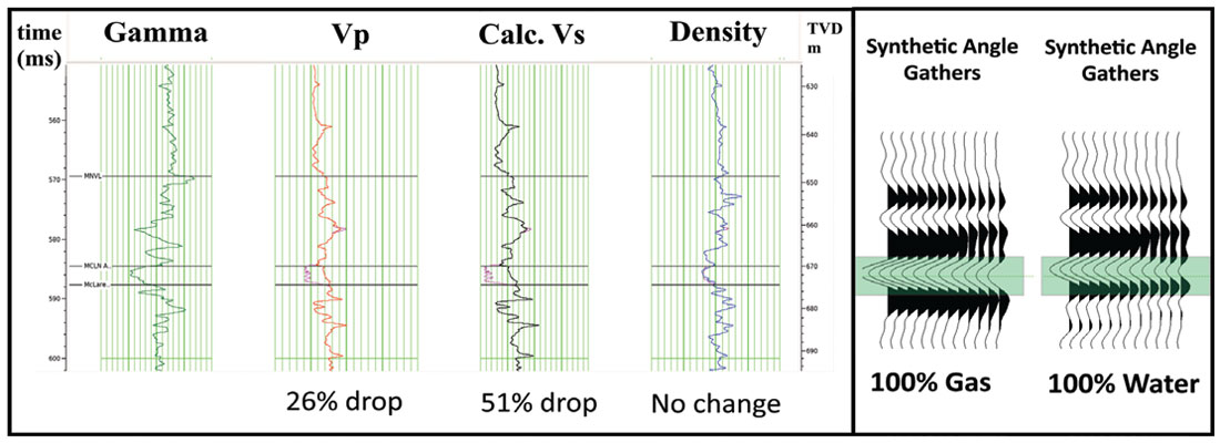
An oil well in the field with a sonic log (V_p) and density (ρ) curves, but no shear sonic log (V_s was calculated), was modified to model the effect of different fluid cases on the logs, such as: 100% water, 100% oil, 100% gas, and varying gas interval thicknesses. The modeled effect of the 100% gas case was consistent with a class 4 AVO response for low impedance gas sands (Castagna and Swan, 1997), with P wave velocity dropping 26% in the gas zone and the S wave velocity dropping 51% (Figure 1).

Fig. 01 — Figure 1. (A) The V_p, V_s, density, and gamma logs for the modeled well. The curves for the 100% gas case are plotted on top each curve in pink. (B) The Zoeppritz calculated synthetic for the wet and 100% gas cases.

The modeling and cross plot results indicated that the gas could be isolated and identified so the gathers were re-processed for AVO compliance. To be ‘AVO compliant’ the relative amplitudes of seismic traces must be restored and preserved, the reflectors must be positioned properly (no post-stack migrations), and noise must be removed. The workflow for this data also included 5D interpolation to reduce noise and regularize the data for the Kirchhoff Pre-stack Time Migration. After processing, the CMP gathers were stacked into 3x3 supergathers to reduce random noise in the far offsets and muted to eliminate residual multiple energy. The supergathers were converted from time-offset to time-angle of incidence and input into Hampson-Russell’s pre-stack simultaneous inversion workflow. This workflow generated the Intercept, Gradient, P Impedance, S Impedance, Density, λρ, and μρ seismic volumes used in the study.

Discussion

The following is a comparative study of the different methodologies used to illuminate a gas cap in seismic data. The methodologies can be categorized as:

Post-stack amplitudes and attributes
Reflective AVO analysis
Pre-stack Seismic Inversion using Acoustic Impedance versus Shear Impedance cross plots and Lambda-rho versus Mu-rho cross plots

Post Stack Attributes

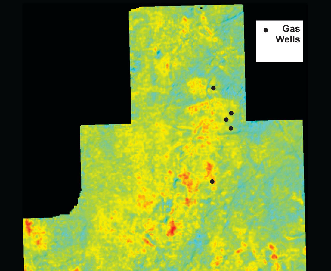
Attribute analysis of the post-stack seismic data showed no appreciable correlation between amplitude and the presence of gas. A time slice showing amplitude at the top of the reservoir had a correlation of 26% with the wells within the seismic survey (Figure 2). Instantaneous frequency, instantaneous amplitude, dominant frequency and sweetness had similar correlation coefficients, with the best result obtained through spectral decomposition.

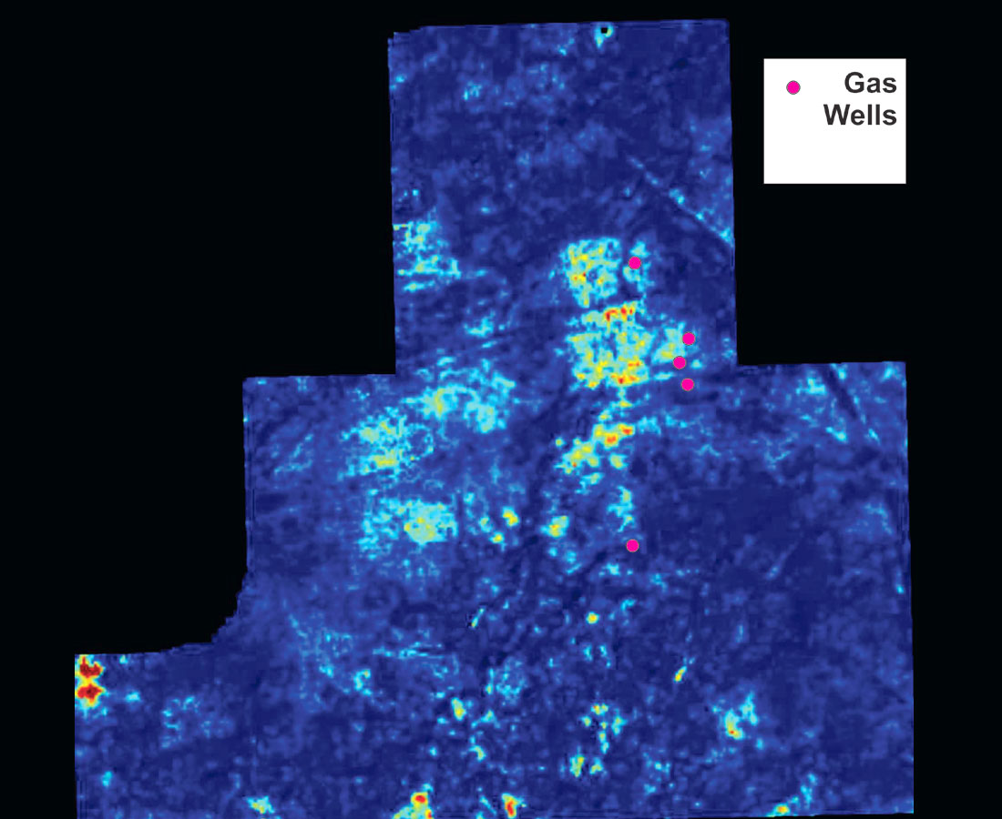
Fig. 02 — Figure 2. A horizon slice through the seismic volume showing the amplitude at the top of the reservoir. (Data courtesy of Arcis, a TGS Company).

A discrete Fourier transform run over the reservoir with a window length of 30 ms, a nyquist frequency of 250Hz, a 20% cosine taper, and a frequency range of 10-100 Hz generated a tuning cube that sliced through time and frequency. The highest correlation to well control (45%), was given by a horizon slice at a frequency of 40 Hz, at the top of the reservoir (Figure 3). It was determined at the end of this analysis that post-stack attribute methods would be of limited use in fluid discrimination in this pool.

Fig. 03 — Figure 3. A horizon slice showing the amplitude at the top of the reservoir through the 40Hz volume. (Data courtesy of Arcis, a TGS Company)

Reflective AVO Analysis

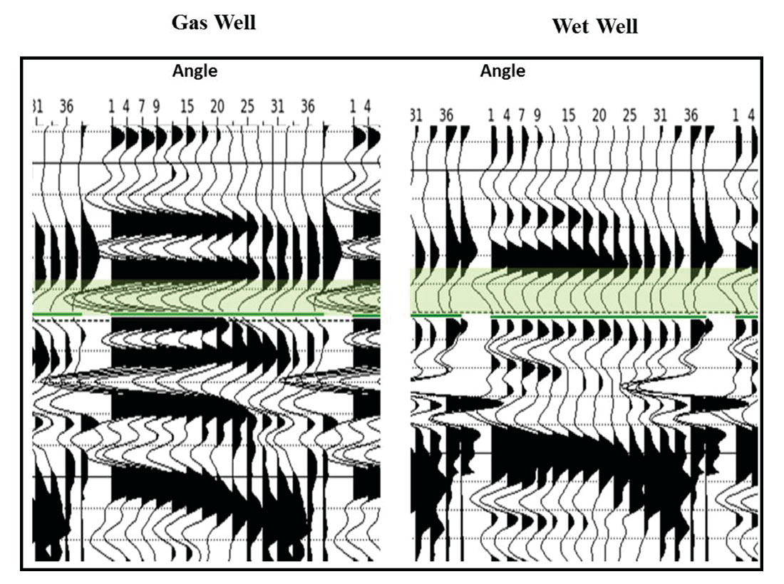
Gas saturated sand in the reprocessed angle gathers demonstrated a class 4 AVO response, with a bright trough at the top of the reservoir dimming with offset. In Figure 4 an angle gather at a gas well is compared with an angle gather at a wet well, showing the anomalous change of amplitude with offset in the presence of gas.

Fig. 04 — Figure 4. The angle gathers over a gas well and a wet well, showing the change of the amplitude with offset in the presence of gas. The trough at the top of the reservoir is highlighted in green. (Data courtesy of Arcis, a TGS Company)

The goal of cross plotting is to separate different lithologies and fluid types from a background trend composed of reflections from water bearing sandstones and shales. Anomalous points off the background trend may represent oil and gas bearing rocks (Chopra, Alexeev, and Xu, 2003). When the V_p/V_s of the background trend is approximately 2, the top and base of a gas sand interval will separate into distinct zones as defined by Castagna and Swan (1997). According to their classification, the top of a type four gas sand should be located in the low gradient, negative intercept zone in the cross plot space. To test this, an inline over the gas cap from the calculated intercept and gradient volumes was cross plotted (Figure 5).

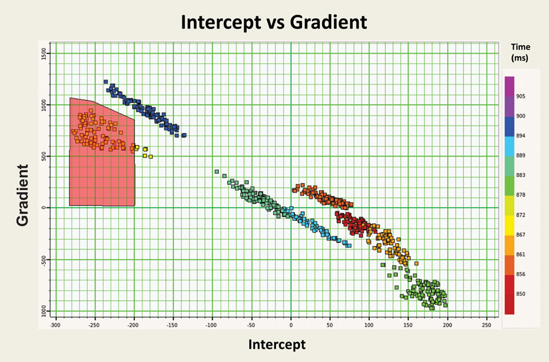
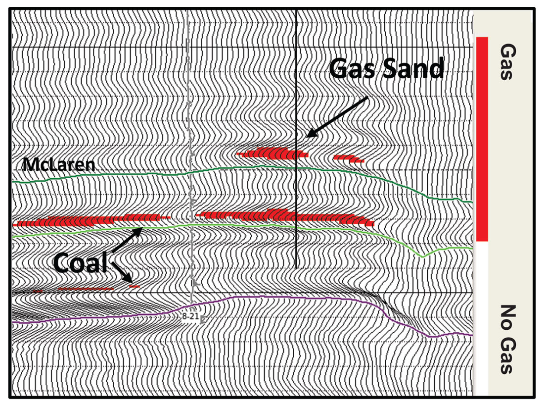
Fig. 05 — Figure 5. The Intercept-Gradient cross plot showing the separation of gas sand, coals, and carbonates from the mudline. Data has been filtered to include only peaks and troughs. (Data courtesy of Arcis, a TGS Company)

The gas zone separated from the background mud rock trend with intercept values below -200 and gradient values below 1000, consistent with the type 4 AVO anomaly. The gas zone identified in the cross plot space was mapped onto the seismic volume (Figure 6). Coals, which occur in abundance in the lower Mannville Sparky and Lloydminster formations, overlapped the gas sands in the negative intercept/ low gradient cross plot space. As a result the regional Sparky and Lloydminster coals were defined in addition to the McLaren sands in the seismic volume.

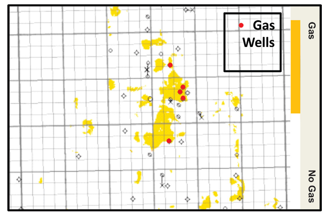
Fig. 06 — Figure 6. An Inline showing the gas sand and coals as defined by the Intercept-Gradient cross plot. (Data courtesy of Arcis, a TGS Company)

The absence of coal within the McLaren formation means that a horizon slice, averaged over a 10 ms window centered on the McLaren should show only the predicted gas sand distribution (Figure 7). The predicted gas-cap was present in almost all of the gas wells and the correlation of the gas/no gas prediction to the wells was 93%. The intercept gradient method tended to over-predict the distribution of gas, with gas estimated below the depth of the oil-water contact in several places.

Fig. 07 — Figure 7. A horizon slice at the top of the reservoir showing the zone defined by the Intercept-Gradient cross plot as a gas saturated sand in yellow. (Data courtesy of Arcis, a TGS Company)

Inversion Attributes and Cross Plotting

Seismic inversion is a non-unique process which involves transforming seismic reflection data into quantitative rock properties such as Acoustic Impedance or Elastic Impedance. It is non-unique because the parameters (V_p, V_s, and density) calculated from the reflective seismic data are influenced by many rock and fluid variables.

The benefits of seismic inversion are:

AVO attributes are converted to physical properties that can be compared directly to well log data
Data is broader band due to the addition of lower frequencies and the reduction of wavelet effects
Wavelet represents rock (geological) layers and not rock interfaces
Can be calibrated to well data
Random noise is attenuated
Interpretability of seismic horizons is improved

The inversion utilized within this project was Hampson-Russell’s Pre-stack Simultaneous Deterministic inversion. Deterministic inversion constrains the solutions by using a low frequency model built from well logs, and the Simultaneous Inversion provides additional constrains by incorporating a user defined linear relationship between V_p, V_s, and density.

Initial analysis utilized the Acoustic Impedance – Shear Impedance or I_p-I_s cross plot for the well data. The raw well log impedances (no upscaling was applied) were cross plotted (Figure 8) to identify the gas sand zone. Raw well data is useful as it provides the best case situation in any area. If the AVO effect is not illuminated with raw well data then it is not apparent within that geological setting.

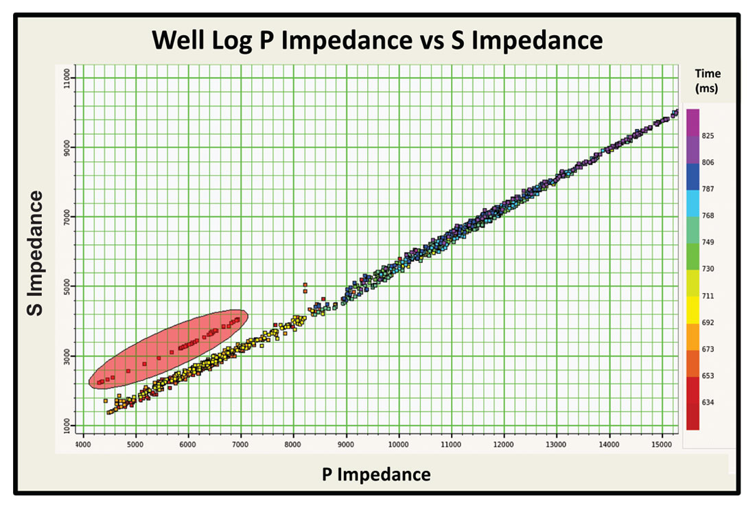
Fig. 08 — Figure 8. The I_p-I_s cross plot for a gas well (calculated V_s). (Data courtesy of Arcis, a TGS Company)

The linearity of the background trend and the good separation of the gas sands in the cross plot is due to the equations that were used to estimate the shear sonic log. The shear log was estimated using the Castagna et al. (1985) mud rock line and the Greenburg-Castagna (1992) iterative method over the reservoir zone. Shear sonic logs do exist outside of the gas cap, and the above estimation method has shown to be extremely accurate for log prediction, just slightly over estimating shear velocities in the unconsolidated wet/oil saturated sand.

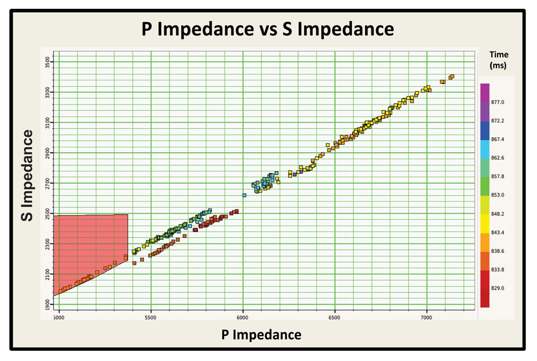
The I_p and I_s volumes from the seismic inversion were then cross plotted (Figure 9) showing good separation of the low impedance gas sands from the background Mannville trend and the less rigid Colorado shales. The separation was not as clear as the well log plot due to tuning and the thinness of the reservoir.

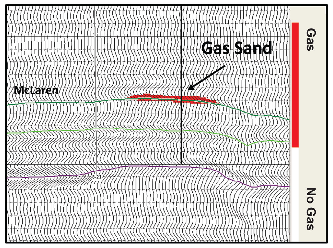
Fig. 09 — Figure 9. The I_p-I_s cross plot of the inverted seismic volumes near a gas well. Data has been filtered to include only peaks and troughs. (Data courtesy of Arcis, a TGS Company)

The gas zone identified in the cross plot was mapped onto the seismic volume (Figure 10). The P- and S-Impedance method was much better than the intercept-gradient method at separating the coals and the gas sands, with almost no coal mapped to the seismic volume in the Sparky or the Lloyd.

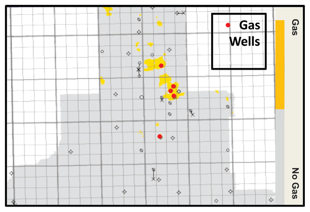
Fig. 10 — Figure 10. An Inline showing the gas sands as defined by the Ip and Is cross plot. (Data courtesy of Arcis, a TGS Company)

A horizon slice averaged over a 10 ms window centered on the McLaren is shown in Figure 11. The predicted gas cap was present in almost all of the gas wells and the correlation of the gas/no gas prediction to well control was 96%. However the southernmost gas cap was completely missing. The large drop in S wave velocity (~51%) in the gas sand affected the accuracy of the Ip-Is method. If the shear velocity remained constant in the gas sand as is seen in classical literature based on consolidated rocks, the separation of gas sands in the low P impedance, high S impedance cross plot space would have provided more accurate separation from the background wet sand trend.

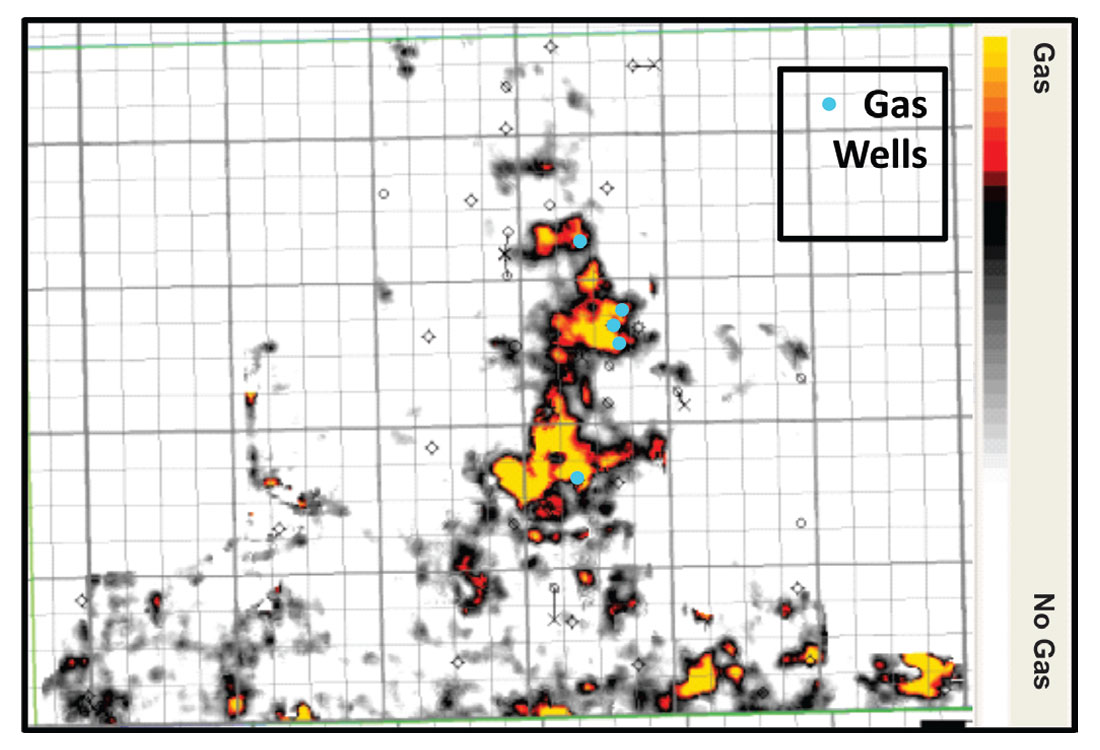
Fig. 11 — Figure 11. A horizon slice at the top of the reservoir showing the zone defined by the Ip and Is cross plot as a gas saturated sand in yellow. (Data courtesy of Arcis, a TGS Company)

Next a horizon slice was averaged over a 10 ms window centered on the McLaren in the V_p/V_s volume calculated during the simultaneous inversion process. This volume predicted a larger gas distribution compared to the impedance cross plot method (Figure 12). The gas wells were all predicted correctly and the correlation of the gas/no gas prediction to all wells was 91%. The southern-most gas cap was present; however the extent of the gas is considerably larger than predicted by the depth structure. This over prediction, and corresponding drop in correlation to well control, is due to the limited offset angles of data at shallow depths. This dataset had a maximum offset of 34°, which was defined by the mute. The minimum offset required to calculate a reliable density volume and, thus separate the velocities from the impedances accurately is 45°.

Fig. 12 — Figure 12. A horizon slice at the top of the reservoir showing the amplitude of the V_p/V_s ratio calculated during simultaneous inversion. (Data courtesy of Arcis, a TGS Company)

Finally the λρ-μρ or Lambda Mu Rho (LMR) volumes were calculated for the well logs and the seismic data, then cross plotted (Figure 13 and 14). The LMR method was introduced in 1997 by Goodway et al. who noted that the wave equation depends not on density and velocity but rather on a ratio of density to modulus, and that velocities themselves depend on a weighted combination of the Lamé parameters. He proposed that the Lamé Parameters: incompressibility (λ), rigidity (μ), and density (ρ) would be more sensitive to changes in fluid and lithology than velocity or density, providing better separation in the cross plot space.

Fig. 13 — Figure 13. The LMR cross plot calculated from the logs in a gas well. (Data courtesy of Arcis, a TGS Company)

Fig. 14 — Figure 14. The LMR cross plot calculated from the inverted impedances. Data has been filtered to include only peaks and troughs. (Data courtesy of Arcis, a TGS Company)

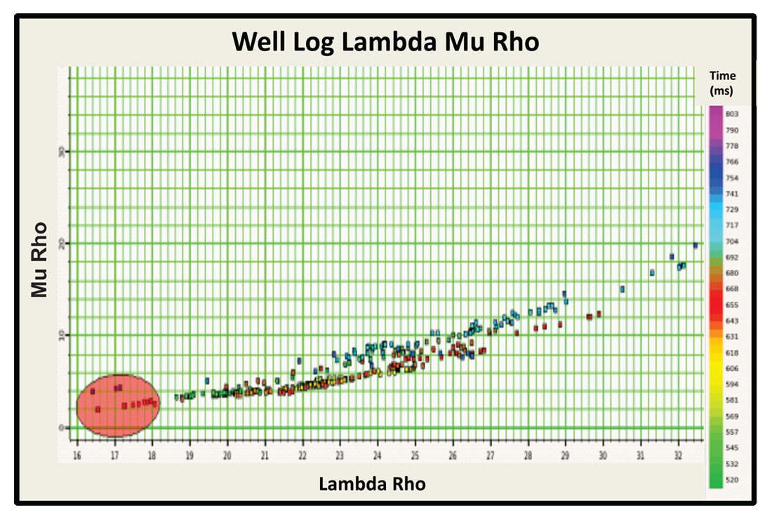
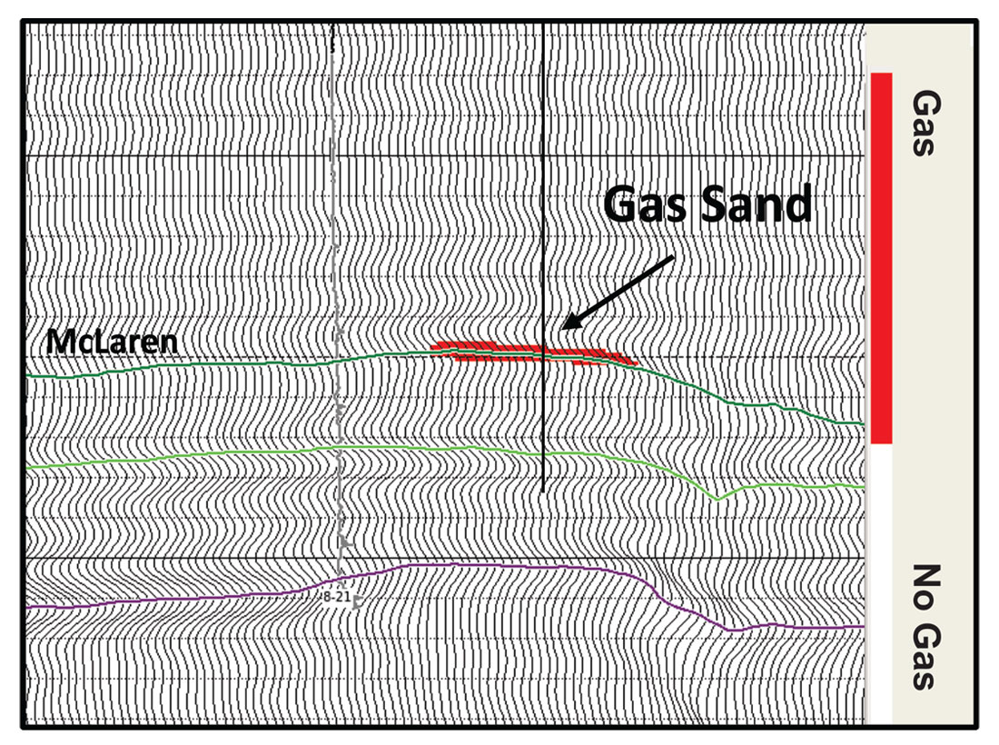
The unconsolidated gas sands seen in this pool have a low rigidity and a high compressibility, which resulted in less separation from the mudline compared to typical consolidated gas sands. The defined gas polygon based on the well log cross plot was projected back onto an inline over the gas cap, defining the gas sands and some coal in the Sparky and Lloydminster (Figure 15).

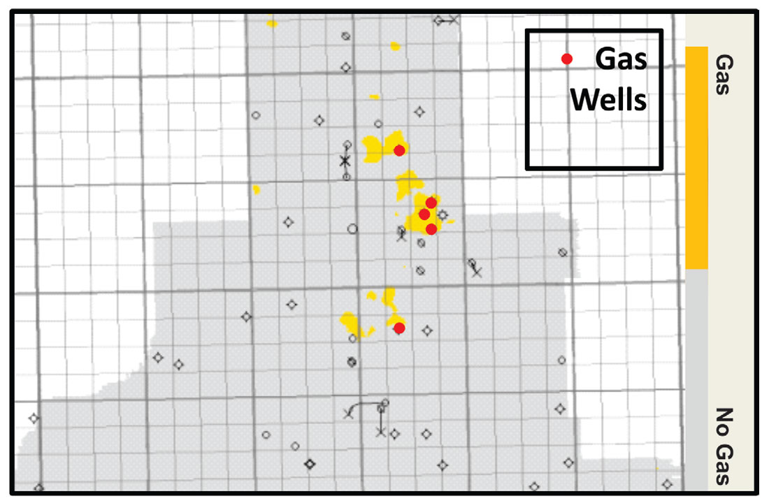
Fig. 15 — Figure 15. An Inline showing the gas sands as defined by the LMR cross plot. (Data courtesy of Arcis, a TGS Company)

The horizon slice averaged over a 10ms window centered on the McLaren (Figure 16) shows a correlation to well control of 100%, with the circular features in the north of the survey caused by karst development in the Devonian rather than gas sands. The position of the predicted gas caps correlates with the structure predicted by depth converted seismic and well control. As the LMR cross plot provided a 100% correlation of the gas/no gas prediction to well control, the horizon slice shown in Figure 16 was used to confirm the location of the four pilot wells.

Further drilling in this area has substantiated the location of the predicted gas cap, with no gas being encountered so far.

Fig. 16 — Figure 16. A time slice at the top of the reservoir showing the zone defined by the LMR cross plot as a gas saturated sand in yellow. This map showed a 100% correlation between the gas/no gas prediction and well control, and was used to confirm the locations of all 2014/2015 wells. (Data courtesy of Arcis, a TGS Company)

The 51% drop in shear wave velocity in the gas sand is abnormal and contrary to classical theory. Since the shear wave travels in only the matrix the shear velocity is supposed to remain constant in a gas sand while the P wave drops, resulting in a change to the V_p/V_s ratio that separates gas sands in the cross plot space. The low shear wave velocity could be due to either a calculation error (though the Greenburg-Castagna method overestimated the shear velocity of the unconsolidated sands in other wells) or the unconsolidated nature of the sands. It is possible that in a low pressure, shallow reservoir, with extremely well sorted and well-rounded grains, the shear velocity does actually drop when the viscous, 12° API oil is replaced with gas. This hypothesis is supported by the inverted Is volume, which also calculated very low shear impedances in the gas sand. This anomalous shear velocity will be the topic of future study.

Assumptions

Hampson-Russell’s inversion software makes several assumptions; that the V_p/V_s ratio in the background model is constant, that Fatti’s approximation is stable for the dataset, that density, I_p, and I_s are linearly related, that there is no NMO stretch in the angle gathers, and that there are no scaling issues. Based on the well log data (only one well in the survey had a shear sonic log) the V_p/V_s ratio from the top of the Colorado to the base of the Leduc ranged from 2.9 to 2.0. The Mannville group ranged from 2.5 to 2.3. Regression analysis suggested that I_p, I_s, and density were linearly related with the regression curves showing a good fit to the data. Initial intercept-gradient analysis confirmed that there were no scaling issues, and any residual NMO stretch was fixed at the zone of interest by applying a mute and trim statics.

Conclusion

Reprocessing modern, high quality seismic for AVO analysis allowed the lateral extend of a thin, unconsolidated gas sand to mapped with a high correlation to well control.

Post stack amplitude and attributes were unable to predict gas with a certainty over 50%. This may be due to the thinness of the sand and the wavelet effects.

The lateral extent of the gas cap calculated by the intercept-gradient method (reflective AVO analysis) had a 93% correlation to the wells. The intercept-gradient method tended to over-estimate the distribution of gas.

The extent of the gas cap calculated by utilizing Pre-stack Simultaneous Deterministic Inversion and cross plotting Shear Impedance (Is) – Acoustic Impedance (Ip) had a 96% correlation to all wells. The I_p-I_s method tended to under-estimate the distribution of gas.

The extent of the gas cap calculated by the LMR method had a 100% correlation to all wells and was confirmed by two pilot wells on the western flank of the high. The accuracy of the LMR method is likely due to the physical dependence of the wave equation on moduli and density instead of velocity and density.

End

Acknowledgements

Thank you to Arcis Seismic Solutions, A TGS Company, for both processing and allowing their data to be used for this paper, with a special thanks to Tricia Cieslewicz, Advanced Processing Geophysicist. Thanks also to Dallas Jones and Peter Wagner at Talisman Energy whose assistance made this paper possible.