Geoscientific Data Adds Value in Unconventional Reservoirs: Statistically Quantified

A dataset of 25 metrics collected from the annual investment reports of 9 public operators in the Bakken Formation is used for statistical analysis of the value of geoscientific data. According to results of this analysis, for each million dollars invested in the geosciences, P90 reserves increase, on average, by 91 +/- 22 mboe after five years for these 9 public operators. Assuming a profit margin of $15/bbl. returns on investment in geoscientific data average 6% for these 9 operators in the Bakken. The Bakken was chosen for this article because it extends into Canada. Operators in other basins see even larger returns (Alvarado, 2016 & 2017).

Under the assumption that through exploration expenses (EXPEX) the cost of geoscientific information can be measured, fixed effects panel regressions with robust standard errors are constructed. These regressions use proven reserves (P90, defined as resources attainable with 90% certainty) as the dependent variable, EXPEX as the variable of interest, and a series of controls accounting for other line items expensed in the EXPEX account. Using the coefficients of these regressions, the ceteris paribus (everything else held constant) effect of investments in geoscientific information on P90 is quantified.

Introduction

In 2014, approximately 12% of the 8.7 mmbpd produced in the US came from the tight oil Bakken Formation. In the current macroeconomic scenario, where excess in supply and decrease in demand are driving oil prices down, several oil and gas operators are reducing their exploration budgets and workforce, and taking a conservative approach to research and development. However, several industry experts point out that a key component in the economic development of unconventional resources is the understanding of the technical drivers of fluid flow, which can only be achieved by the application of new technologies (Moniz et al., 2011). In this sense, using low commodity prices to rationalize a reduction of capital allocated to exploration and research for unconventional resources may be detrimental for a firm’s long-term value. This paper is motivated to help decision makers quantify the financial returns of investments in geoscientific information for unconventional resources independently of oil prices. The objective is to provide a deterministic economic model using real data that quantifies the average financial return of investing in new technologies.

In this paper, geoscientific information is defined as geological, geophysical, and technical data describing the in situ conditions of a reservoir. Some examples of geoscientific information are seismic imaging, petroelastic inversions, microseismic surveys, FMIs, geomechanical models, acid jobs, and tracers, to name a few. The value of the geoscientific information depends on the cost to acquire this information and its derived benefits. For example, monitoring hydraulic stimulations with multicomponent seismic permits a clear image of the fracture network, thus providing a better understanding of the petroelastic properties of the rock (Barkved, 2004). In this example, the investment is made in a geoscientific project (the acquisition of seismic data) from which geoscientific information (subsurface images) is obtained. Using this information, operators make better decisions that optimize operations (well planning, directionality, completion depth), leading to higher financial returns.

Managers in the industry use Value of Information (VOI) exercises as the standard procedure to evaluate the need of technical information (Bailey et al., 2011; Borison, 2005; Strunk, 2006). VOI exercises are deterministic calculations from the real options theory where, in its simplest terms, information is valued as the difference between the value of an asset with current and future information. However, VOI exercises cannot be used to quantify the value of geosciences on average for public shale operators. This is so because VOI exercises are subjective, they depend on the risk aversion of the decision maker (Eeckhoudt and Godfroid, 2000), they require a very specific definition of the desired information (Bailey et al., 2011), and furthermore these exercises require defining uncertainty through probabilistic functions backed by historical data (Strunk, 2006). In this paper, returns from investments in geoscientific information are quantified on average for public operators with key assets in the Bakken. Instead of making use of the real option theory and VOI exercises, this work uses econometrics and statistical regressions on a dataset containing several corporate metrics describing the past 20 years of exploration activity.

Methodology

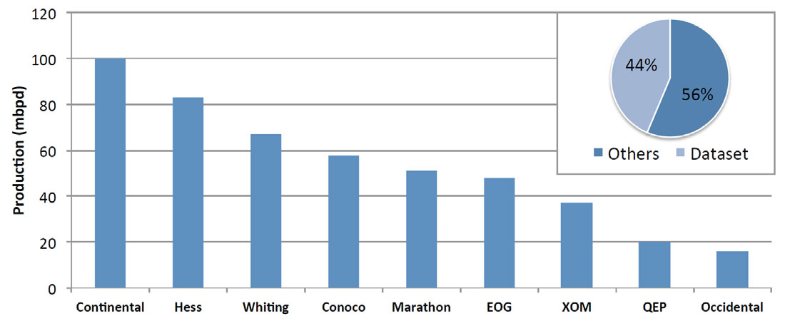
The findings presented in this paper are the result of equity research and statistical analysis. First, in the equity research part, the annual investment reports of the top public producers in the Bakken Formation as of 2014 were investigated (Figure 1). 25 metrics were collected for each of these operators from 1995 to 2014, which include the 1998 and 2008 downturns, using the investment reports available online to the public through the Securities and Exchange Commission (SEC). Some of the metrics in the dataset capture changes in exploration and development strategies among operators (exploration expenses, proven reserves, acreage, drilled wells, etc.), other metrics describe their business and financial position (enterprise multiples, reserve life indexes, price per flowing barrel, etc.), and some metrics capture macroeconomic scenarios (oil prices, interest rates, time trends). A detailed list of the metrics is provided in Appendix A. The metric of interest in this paper is exploration expenses (EXPEX) because investments in the acquisition of technical information are expensed in this account.

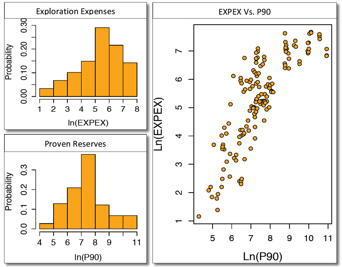
Now, let’s describe the statistical analysis used in this paper. The metrics gathered from the investment reports were organized as a panel. In statistics, a panel is a bi-dimensional array that measures the changes in metrics (X) across companies (i) through time (t). The panel contains 148 observations from 9 public operators. The average EXPEX in the panel is $630 M with a minimum of $4 M, a maximum of $2144 M, and a standard deviation of $572 M. Analogously, P90 has an average of 7318 mmboe with a minimum of 122 mmboe, a maximum of 55946 mmboe, and a standard deviation of 12215 mmboe. Due to the large range in the values of EXPEX and P90, histograms showing the distribution of both metrics in natural logarithmic form are given in Figure 2. Figure 2 also shows a relationship plot showing a clear positive relation between EXPEX and P90. Furthermore, the correlation between P90 and EXPEX for this panel of operators in the Bakken is 0.65, which means that up to 43% of the variations in P90 could be explained by changes in EXPEX (Baltagi, 2011).

A type of multivariate regression called fixed-effects panel regression with robust standard errors is constructed to quantify the effects of EXPEX on Proven Reserves (P90). This type of statistical regression permits quantifying the interaction between variables across companies, addressing any unobserved differences among them (Woolridge 2012; Baltagi, 2011; or Greene, 2012). In short, this type of regression allows us to quantify the relationship between metrics among companies with different budgets, market capitalization, enterprise value or any other intrinsic characteristic. Since each metric is a time series, the metrics are highly correlated and autocorrelated (e.g. the reserves of EOG in 2007 are likely to depend in some degree on its reserves, production, and acreage in 2006). The problem with constructing statistical regressions with autocorrelated variables is that the resulting model tends to underestimate standard errors (Greene, 2012). Hence, a method called the Arellano procedures was used to construct robust standard errors and 95% confidence intervals.

To account for the cumulative effect of investments in the geosciences, finite distributed lag models (FDLM) were used. FDLM are multiple regressions where the lagged values of a variable of interest are also used in the regression equation (Baltagi, 2011; Woolridge, 2012). As an example, it takes time for a pharmaceutical company to find a new cure so the effect of investments in R&D on profits will show up with a lag and will be significant for many years afterwards. Similarly, it can take years for investments in geoscientific information to pay off, so the effects of exploration on other corporate metrics are likely to show up with lags and be significant for several periods afterwards. However, due to limitations in the dataset, a maximum of 5 lags of EXPEX was considered in each model.

Finally, once the relationship between EXPEX and P90 is quantified using the regression coefficients, this information is used in a discounted cash flow model where ROIs are quantified as a continuously compounded interest rate using the following formula (Equation 1):

EQUATION

Where FV represents future value, PV present value, i the interest rate (ROI in this case), and t the number of periods (years).

Results

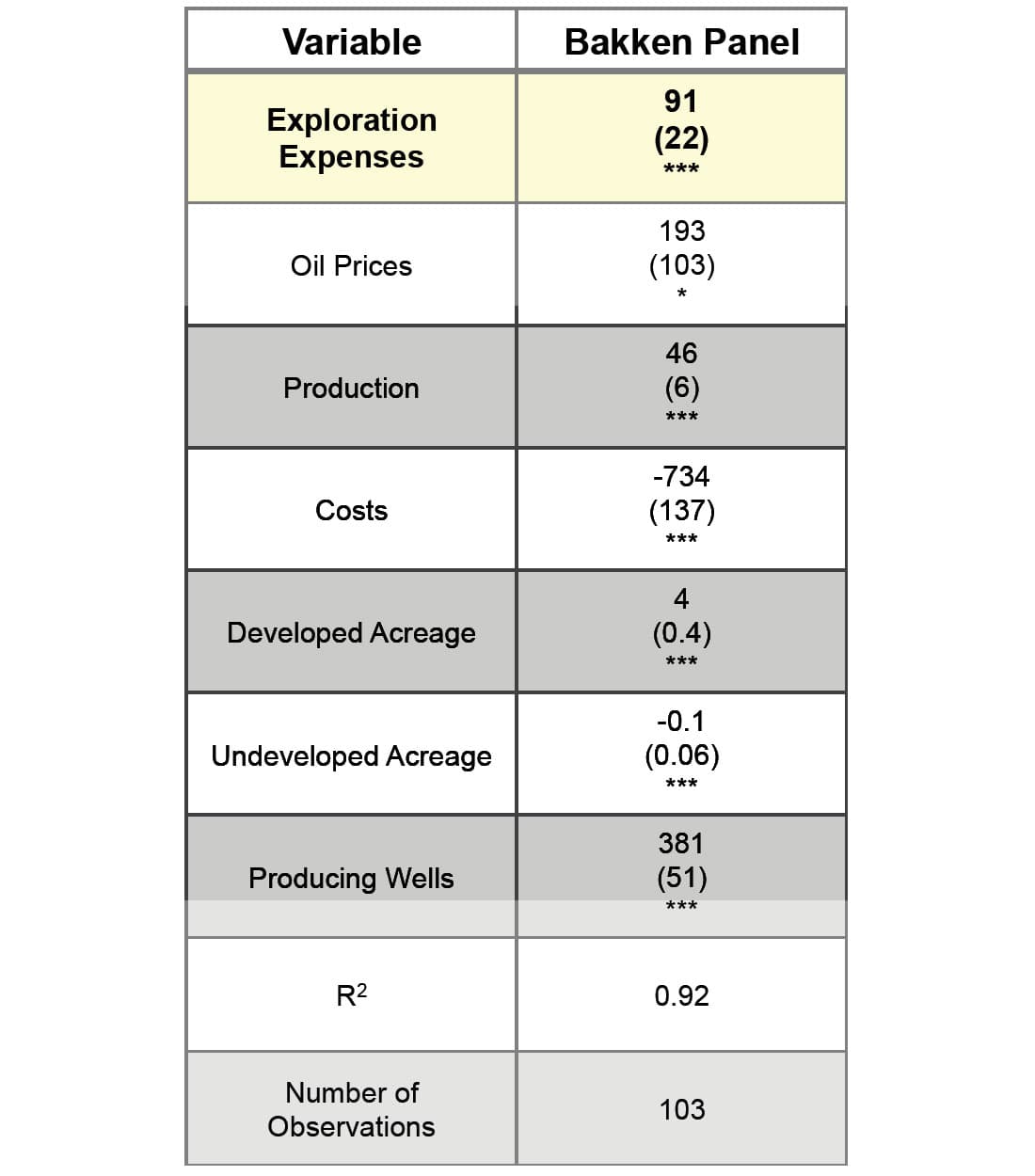
Table 1 shows the regression coefficient of the variable of interest EXPEX (highlighted in yellow) and selected controls obtained from the fixed effects panel regression of P90 vs. EXPEX for the top operators in the Bakken Formation. Under the regression coefficients, the reader will find the standard errors and symbols illustrating statistical significance. The result of this regression can be interpreted as follows: a million dollars invested in the geosciences will increase the amount of proven reserves by 91 +/- 22 (95% confidence interval) thousands of barrels of oil equivalent after 5 years.

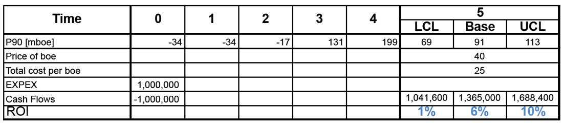
Using this information, a discounted cash flow model is constructed to estimate expected returns on investment. On Table 2, this procedure is illustrated in a practical way. The first row represents the time after investment (in years). The regression models quantified an increment of 91 thousand barrels of oil equivalent with a lower confidence level (LCL) of 69 and an upper confidence level (UCL) of 113 as illustrated on the second row of Table 2. The third row assumes a fixed price of $40/bbl. The fourth row assumes a total cost per barrel of $25/ bbl, leaving a profit margin of $15/bbl. Under these assumptions, geoscientific projects have an average ROI of 6% for these 9 operators.

Conclusions

In this paper, the financial returns from geoscientific information are quantified using panel data econometrics. Specifically, results indicate that $1 MM invested in geosciences increases the amount of proven reserves (P90) by 91 +/- 22 (two standard deviations) mboe on average 5 years after the geoscience investment for the top public operators in the Bakken Formation. Assuming a profit margin of $15/bbl, these increments in P90 attributed to EXPEX can have ROIs as high as 10% under the assumptions stated in this paper.

Given access to time series describing the changes in acreage, production, management, reserves, costs, and type of technologies at a field or basin level, which are often available in annual and/or government reports, econometrics could then be used to quantify the returns from specific exploration technologies (microseismic, tracer data, seismic surveys) across different basins independently of commodity prices.

Acknowledgements

The Reservoir Characterization Project (RCP) from Colorado School of Mines. Tom Davis, Graham Davis, Peter Maniloff, Hortense Viallard.