Good Computer Contouring/Modelling Can Help the Geophysical Interpreter

This is the first in a series of articles on contouring, or modelling, to use the more appropriate term. The purpose of this series is to develop the principles and role of contouring in present day exploration. The first of the four articles discusses basic gridding and triangulation techniques. The second will be about multi-surface contouring, stacking, faults and the handling of fault planes. The third will be a discussion on the uses of contoured data such as reconstructions, mapping pinchouts, mapping with dips from well logs, calculating residuals, volumetrics, cross-sections etc and the last article will be on 3-D seismic and wells.

Gridding and Triangulation Introduction

Computer contouring programs now comply with most of the requirements which are important when contouring:

• honour the given data
• appear to be contoured by hand
• handle faults properly
• have three dimensional rigour
• work either in time or depth
• be fast and economical

As more and more data are being interpreted on workstations, and the use of visualization is increasing, there is a greater demand for contours in digital form. Contours are utilized by all members of the team. The geologist and geophysicist for structural purposes, the engineers for economics, the drilling engineer for developing the drilling plan, the development engineer for selecting the next location and the reservoir engineer for reservoir simulation.

Companies also are looking for ways to reduce costs and get more information from the data at the same time. Computer assisted contouring allows the geophysicist to evaluate more prospects in a given time period and reduces the risk on a prospect by permitting the explorationist to look at a greater number of scenarios.

In the past, companies operating in the Western Canada Basin have utilized single surface maps, without faults. With the advent of the computer, however, they can now consider multi-surface contouring with faulted surfaces and produce more maps with more sophisticated interpretations of the data. Geostatistics, the art of correlating one attribute with another, is becoming increasingly popular, but still needs a quality contouring package. As companies explore in the Foothills and internationally, contouring packages which properly handle both normal and reverse thrust faults are essential. Powerful visualisation programs are now available, but they are only as good as the surfaces they are displaying. An understanding of the basics of modelling is essential if the speed and power of the computer are to be exploited effectively.

Interpolation: The Basic Problem of Contouring

Beginning with the earliest seismic shooting, the goal has been to create a multi-surface model of the subsurface and display it with a series of maps. Representing three-dimensional surfaces on a two-dimensional surface has always been a challenge, even when an unlimited amount of data are available. When data are limited, the problem of representing that surface becomes more difficult. The location of the surface between the data points must be derived from the existing data using interpolation.

Interpolation is a relatively simple but time consuming task for the human brain. Interpolation by a computer is much faster, although it is more difficult to emulate the subjective and aesthetic characteristics of human contouring. So contouring becomes a trade off between speed and aesthetics. How much time do you want to spend to evaluate that high, one minute of computer contouring or one day of your geophysicist's time?

Faults complicate the contouring process because they destroy the continuity of surfaces being contoured. When contouring faulted surfaces by hand, mentally we compensate for the vertical displacement and copy shapes across the fault. A computer program should be capable of copying shapes across faults. This ability is termed vertical interpolation.

The essence of contouring is the interpolation of data, both horizontally and vertically. Interpolation is the mathematical art of estimating. An interpolation process calculates the value of a surface between known values. It is an art in the sense that there is no limit to the number of formulae that can be conceived and the choice of formula includes a number of subjective criteria: Does the map look pleasing? Does it come close to how I would do it by hand? Is it reasonable?

Only two fundamental procedures are used by computers to generate contours: indirect or gridding techniques and direct or triangulation methods.

Indirect Technique (Gridding)

This technique uses the original data to calculate a second set of points. This second set of points follows an orderly grid pattern and replaces the original data. All subsequent calculations draw contours using the gridded data points. The purpose of using this technique is to simplify the subsequent steps in contouring by making the geometry more manageable.

The grid can be oriented in any direction, and the size of the grid determines the extent of the contours. The contoured map can have a different look for different orientations.

Gridding always involves four steps:

1. Select a grid cell size and an origin for the data. A grid node is formed at the corners of each cell.
2. Sort the original data points according to their X-Y locations.
3. Select neighbours from the original data points for each grid mode.
4. Create a second set of values located at the grid nodes using the set of neighbours from the original data set.

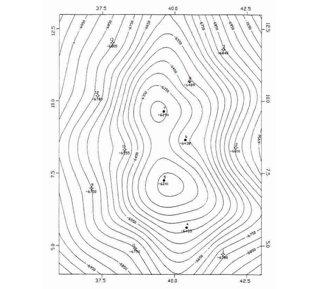
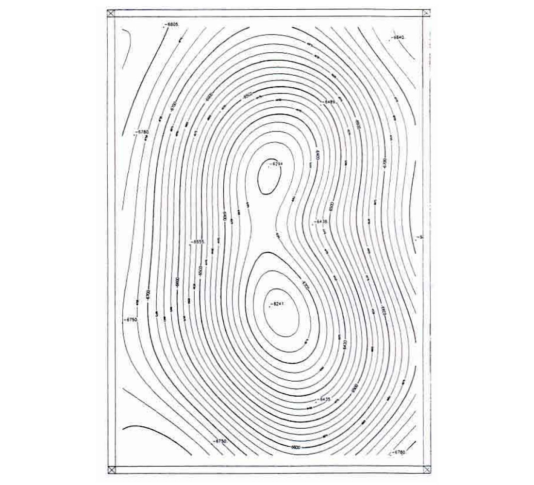
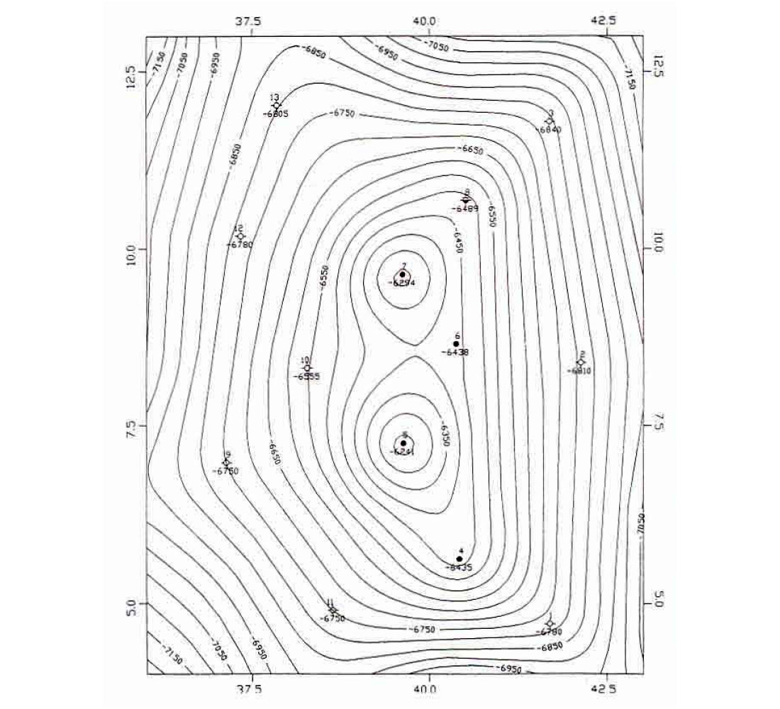
The last two steps are where numerous schemes have been developed to make maps that are aesthetically pleasing and honour the data points as much as possible. Three examples of these schemes are shown in Figures 1-3. These examples are from the same data set. The interpreter has to choose which interpolation method to use and which method to use for selecting neighbours. If there are 5 ways of selecting neighbours and 10 ways of interpolating, the user can get 50 different maps for each grid cell size. With gridding it is easy to ensure that any contour line drawn through a grid honours the grid points. However, contour lines that honour the grid cannot be guaranteed to honour the original data points.

Direct Technique (Triangulation)

Triangulation was the first procedure used in trying to use computers to make contour maps. The reason was because surveyors triangulated when making topographic maps and most of us used triangulation when learning to contour by hand.

Direct contouring techniques (triangulation) interpolate values along a pattern which is derived from the pattern of the original data. The values of the original data are preserved in the pattern and are kept throughout the subsequent processing which ensures that the contours will honour the original data.

Triangulation requires the selection of neighbours; however, the task of determining neighbours is finished when the data has been triangulated. The resulting triangulation has the following characteristics:

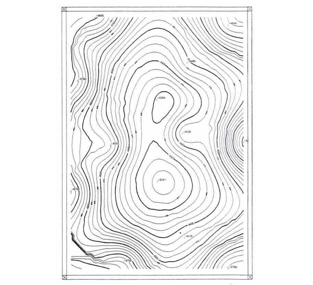
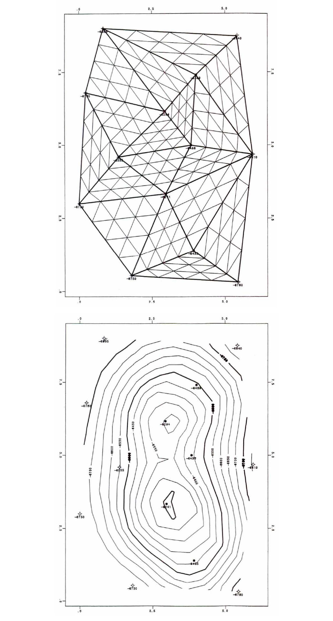
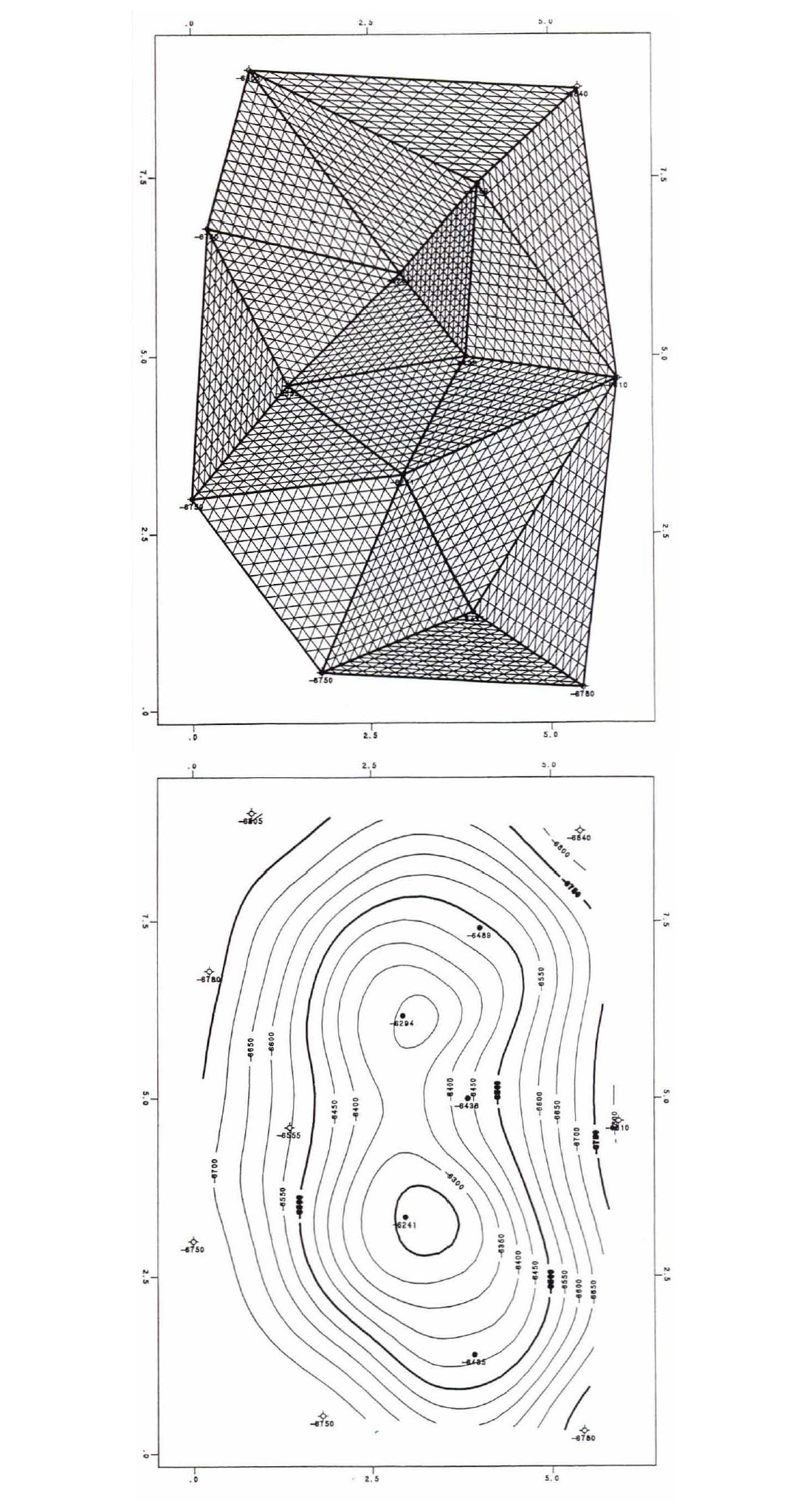
1. The X-Y data set containing n data points has been broken into a set of triangles. Figures 4-6.
2. These triangles have data points at each vertex, are as equilateral as possible and the contours do not change with orientation. These triangles are called Delaunay triangles.
3. In large random data sets, each point will have an average of six neighbours. If the points are not located randomly, e.g. 2D seismic data, some points will have more than six neighbours, others will have fewer.
4. Contours are not calculated beyond the perimeter of the original data. Figures 5 and 6 are examples of triangulation. Smoothness, i.e. subdivision of the original triangles, is the only variable involved. The interpolation is the same regardless of smoothness.

Summary

Only two techniques are involved in data interpolation: gridding and triangulation. The fundamental difference between the two is that the triangulation method honours all data points, and gives the same interpolation regardless of smoothness. The gridding method is more flexible, but does not always honour the data points.

Many contouring programs and visualisation techniques are now available to the desktop interpreter. This will lead to increased exploration benefits from contouring well tops, seismic times and attributes of potential field data. No matter what level of sophistication you deal with, there are still only two fundamental choices of contouring methods to be made, and that is the choice between the indirect (gridding) or the direct (triangulation) technique.