Good Computer Contouring/Modelling Can Help the Geophysical Interpreter – Part Two

The first article of this series discussed the differences between gridding (indirect) and triangulation (direct) as methods of contouring. The examples were based on well data and only one non-faulted surface was contoured. In this section we first discuss the contouring of several surfaces followed by a discussion of a method to handle faults.

Multi-surface Contouring

Most formations were nearly horizontal when deposited and the formations were sub-parallel to each other. Even though geologic forces have deformed the original structures, many suites of surfaces exhibit similar features. This is the familiar geologic principle of conformity that can be applied when contouring several surfaces simultaneously.

The technique is as follows. Calculate isochores, the vertical distance between surfaces, where possible. Interpolate or extrapolate these values over thy entire map for all isochore intervals. Add or subtract the calculated isochore values from known data to reconstruct a complete set of Z values at all data points. This step is called 'stacking'.

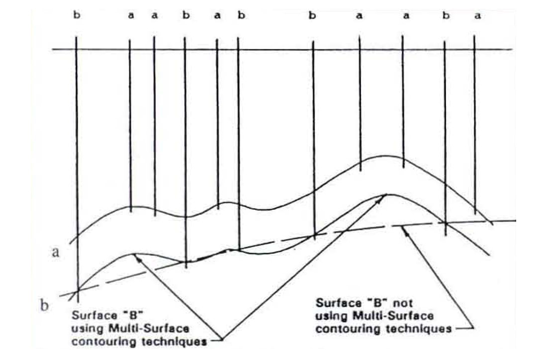
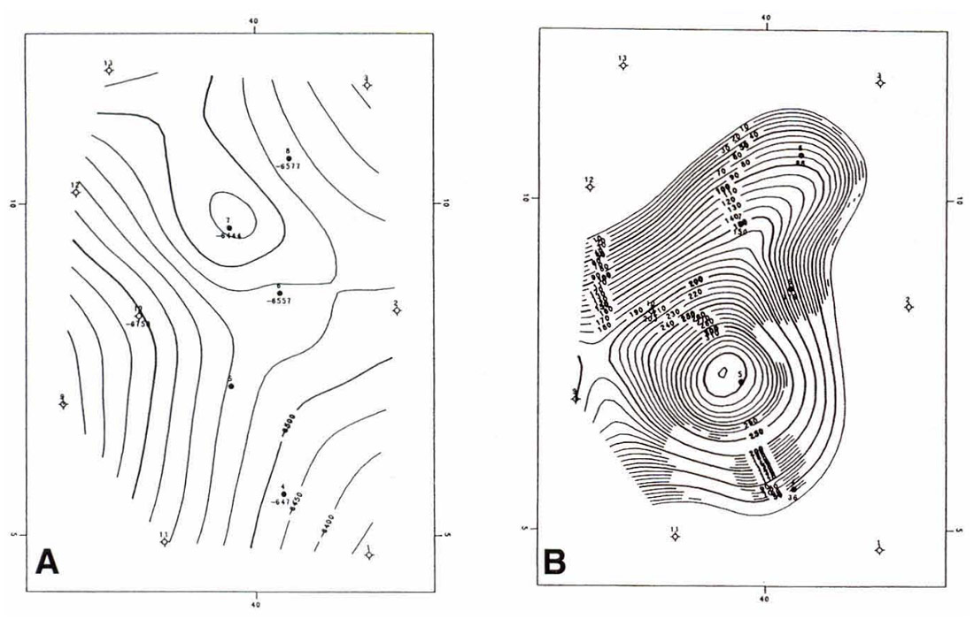
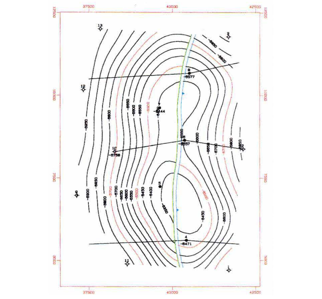
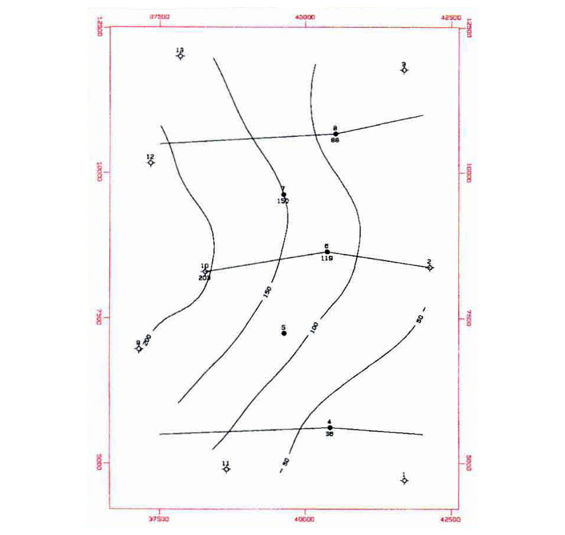
Figures 1 and 2 illustrate the effect of multi-surface contouring. In Figure 1, only five wells penetrate to surface B. If multi-surface contouring is not used, the less conformable dashed line is the result. Figure 2(a) represents surface A. Figure 2(b) represents surface B using multi-surface stacking. Note how the surfaces are conformable. Figure 2(c) shows surface B without stacking. There is a distinct difference in the shape of the B surface if stacking is not used.

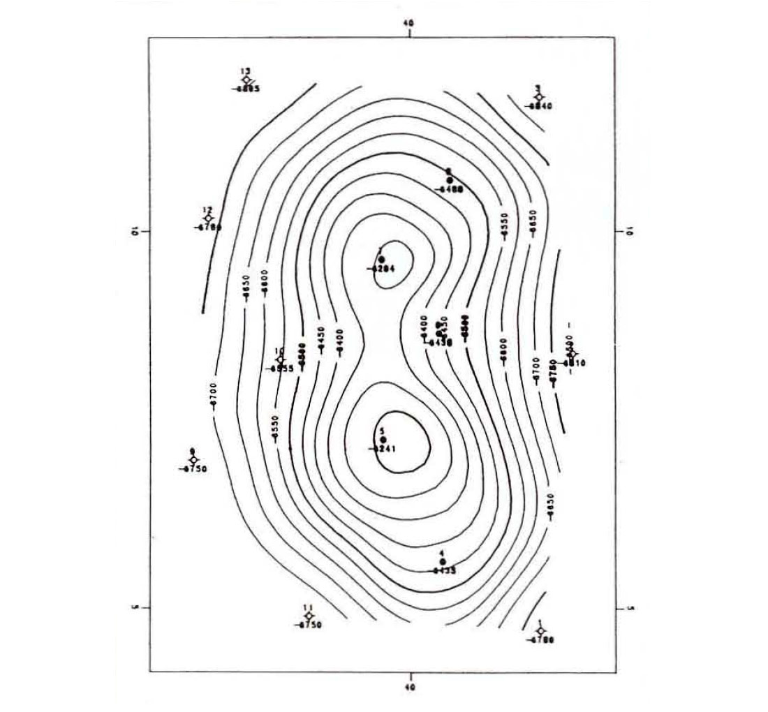
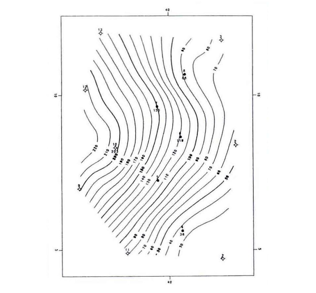
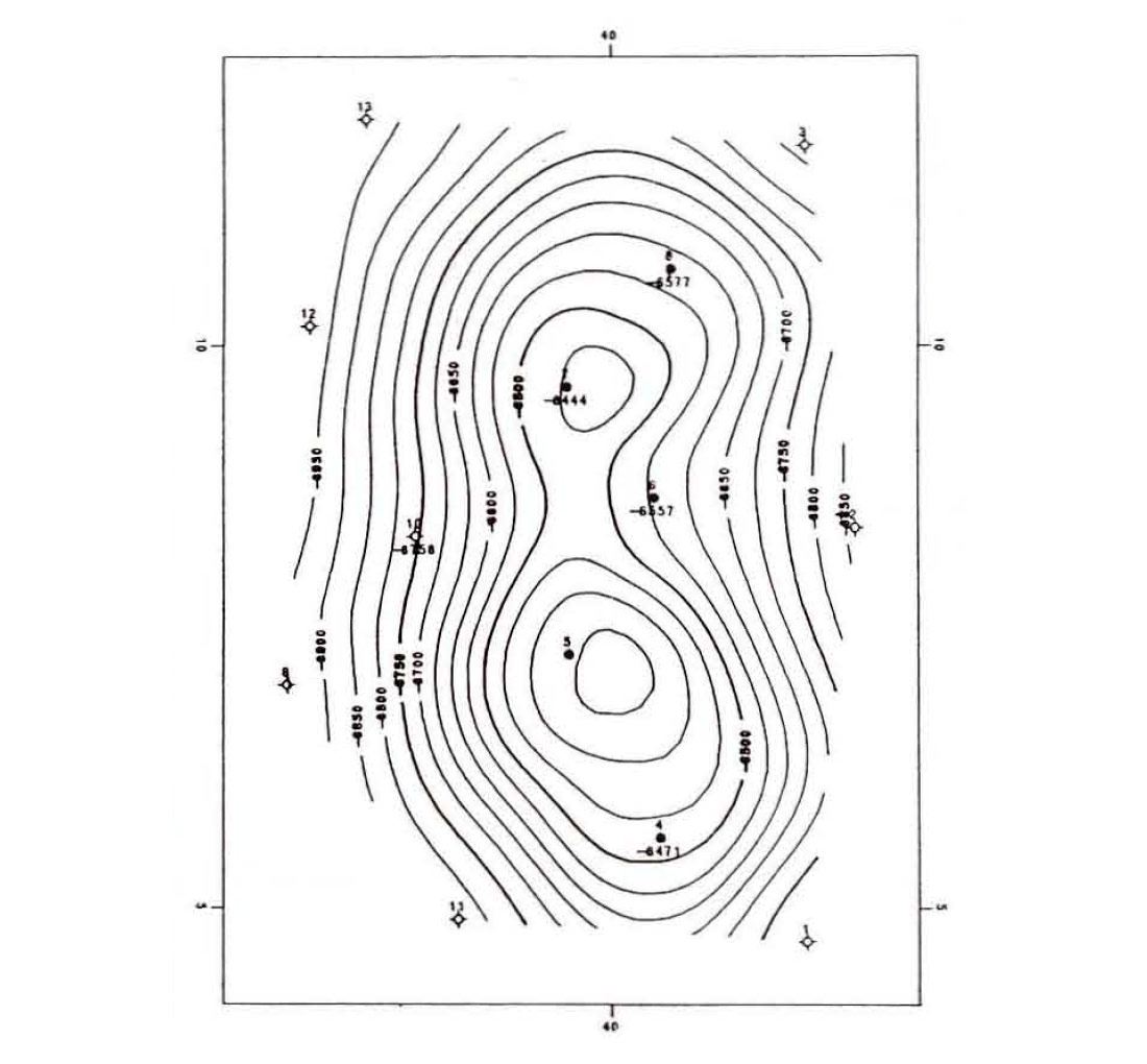
An even more startling difference occurs in the isochore maps. Figure 3(a) was determined by subtracting Figure 2(b) from Figure 2(a). Figure 3(b) was determined by subtracting Figure 2(a) from Figure 2(c). It is obvious that multi-surface contouring provides a more accurate representation of the subsurface.

Fault Handling

To perform a comprehensive interpretation of a data set, a contouring package that manages faults is essential. One method of managing faults is described below.

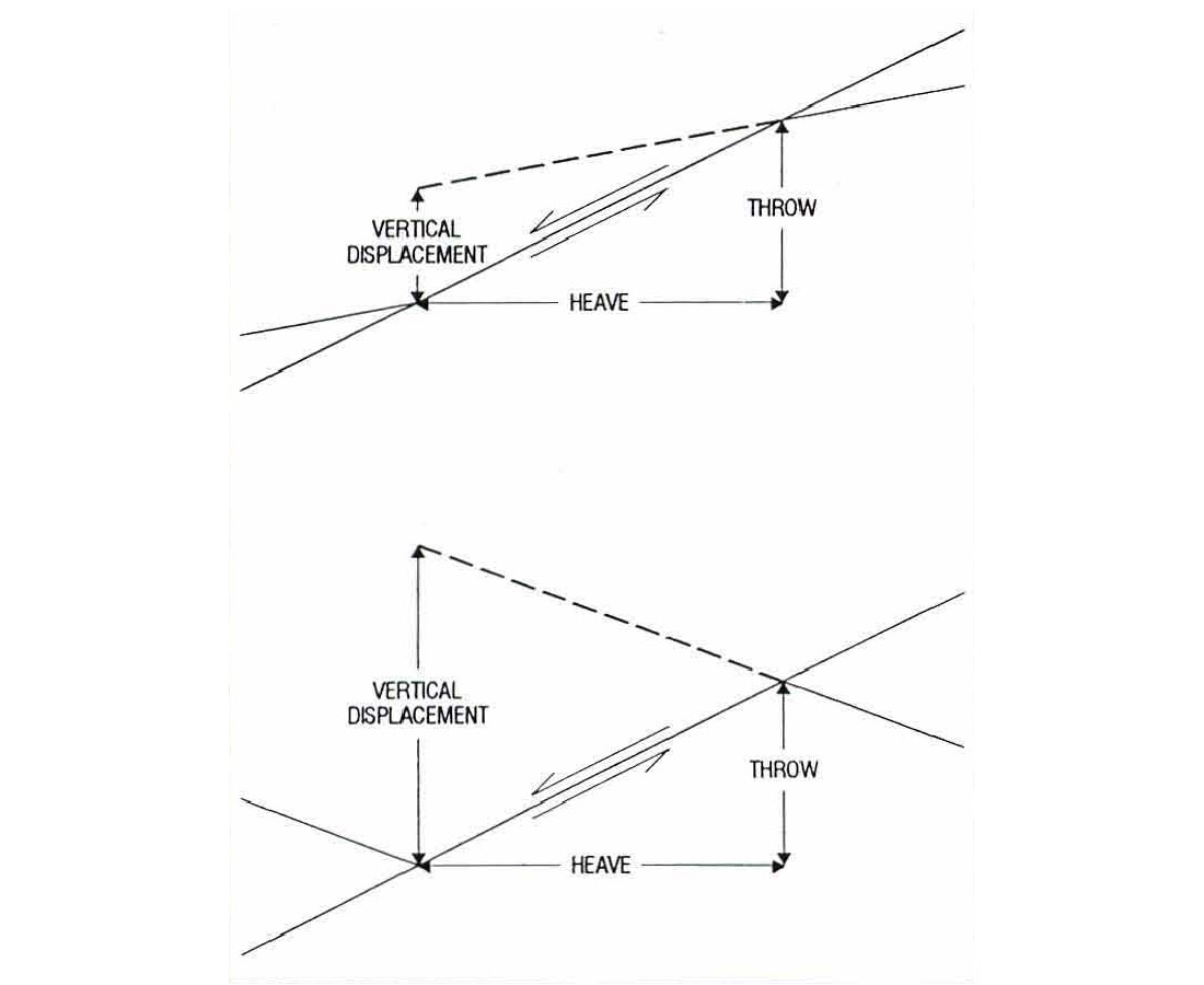
Fault systems are treated as sets of three-dimensional blocks containing geologic markers that were once continuous surfaces. The boundaries of these blocks are the fault surfaces and are treated as contourable surfaces. To model such systems successfully, three or more X-Y-Z points for each fault surface are required, along with fault vertical displacement. Fault vertical displacement, heave and throw are illustrated in Figure 4. Fault vertical displacement is not synonymous with throw. In Figure 4 the throws are the same but vertical displacement is not.

Faulted data are treated the following way:

1. Move the fault blocks vertically and in the proper restoration sequence by the amount of fault vertical displacement.
2. Interpolate and stack the isochores.
3. Move, or rebreak, the blocks back to their present day faulted position and contour the data.

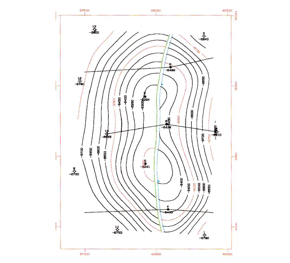
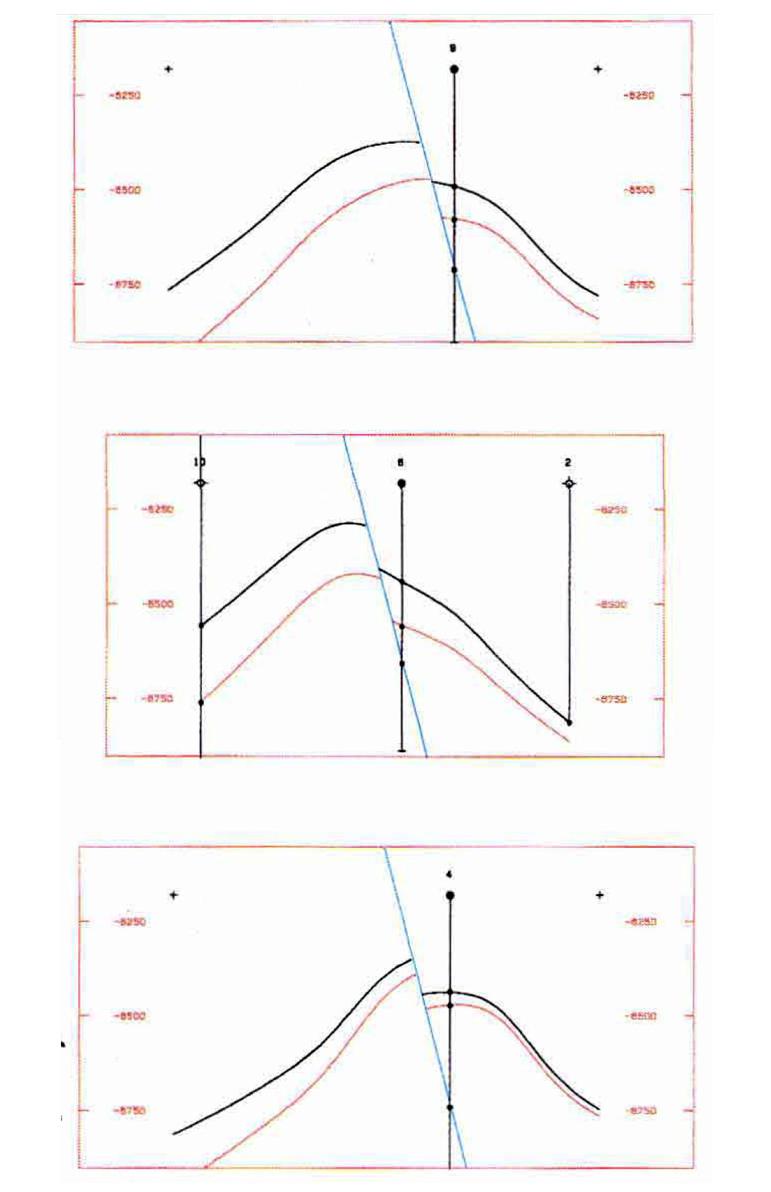
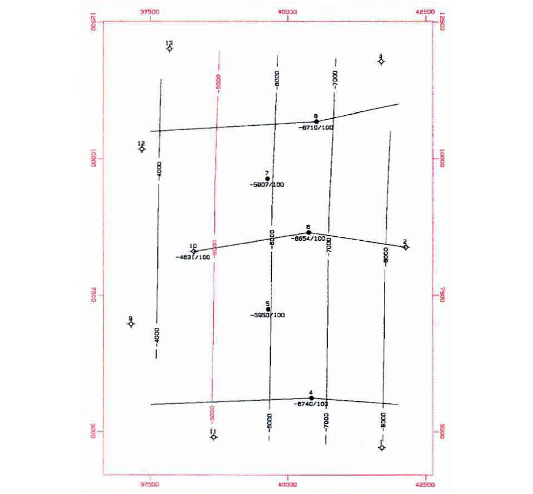
well tops in Figure 5(a) and 5(c). Note that Figure 2a and Figure 5a are the same data set except a fault, with 100 feet of fault vertical displacement, has been introduced into Figure 5. Cross sections through the data Figure 5(b) illustrate that the shape of the structure has been preserved across the fault. Note in the cross sections that the thickness of the formation is identical on both sides of the fault. In Figure 6, the isochore was calculated and contoured. The top of formation and the isochore were stacked to determine the bottom of formation. The surfaces to the right of the fault were then shifted vertically downward by the amount of fault vertical displacement and contoured. Fault traces were then generated by calculating the intersection between the top and bottom of formation and the fault surface.

The stacking method requires formation tops or times, fault location and fault vertical displacement as input. Also required is the correct sequence of restoration. The result is a set of contoured maps for each horizon, contours of the fault plane (Figure 7), and the intersection line between the fault plane and the top or bottom of formation. The method can be applied to normal faults, reverse faults and strike slip faults where the fault vertical displacement can vary from positive values through zero to negative values.

Contours Below Thrust Faults

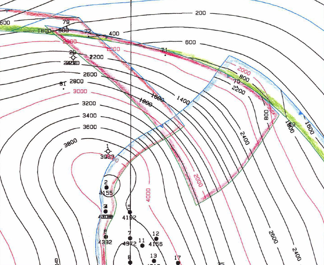
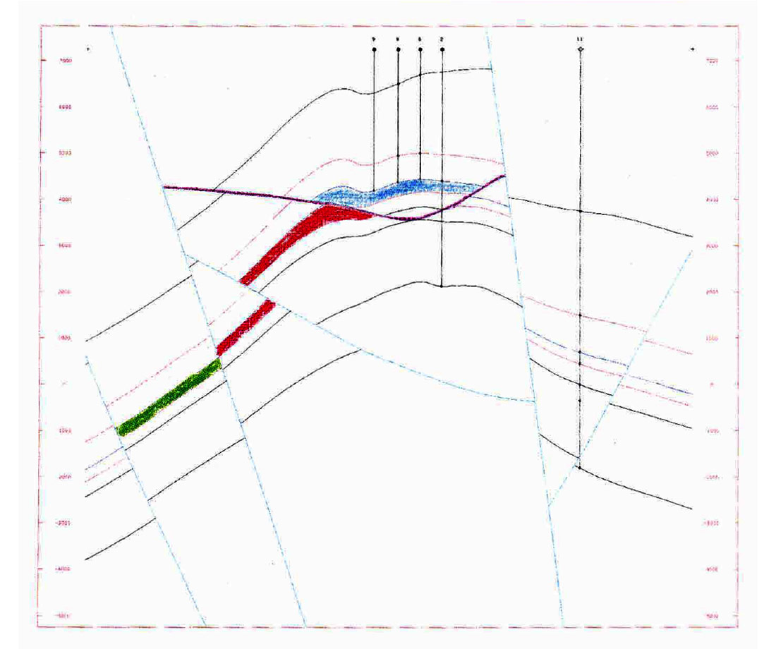
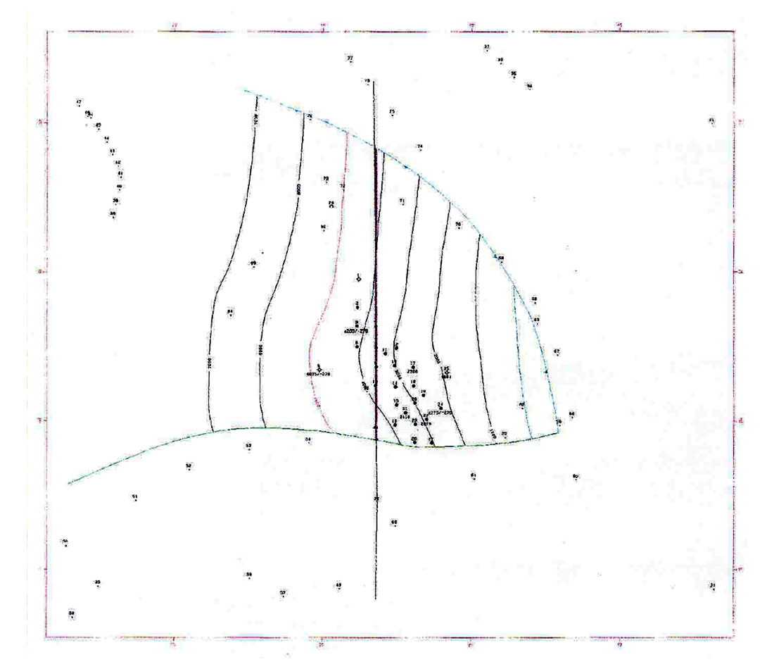
One interesting result of this method is that contours below a thrust fault are displayed along with the values above the fault. On the front cover, the contours do not overlap because the faults are normal faults. Contrast this map with Figure 8, a thrusted area in Wyoming called the Quealy Dome (Stone, 1995). Figure 9 is the north-south cross section through the Quealy Dome. In the central portion of Figure 8, the contours above and below the reverse fault are obvious because of the separation between the contours. On the other blocks the contours are co-linear and are less obvious. The blue block has been thrust northward over the orange, red and green blocks. The orange block has been thrust northeast-ward over the red and green blocks and the red block has been slightly thrust NNE over the green block.

Fault Planes

Another result of the method is contours on the fault planes. In Figure 7, the fault surface is simple and extends throughout the entire map area. However, not all fault surfaces are so planar. Figure 10 shows the contours on the fault at the base of the blue fault block. The fault dips to the west. That portion of the fault plane in the cross section has been colored in purple.

Conclusion

In this article, we have discussed how several horizons can be contoured at one time. The concept of stacking in contouring terms was extended to the handling of faults. The output from the fault handling includes contoured maps of formation tops and bases, isochores and fault planes. The contoured maps show contours above and below fault surfaces. This information forms the basis of the development of the structural history of a prospect, fundamental in hydrocarbon exploration.