Abstract
Microseismic monitoring is an important tool for developing unconventional resources such as shale gas and understanding the geomechanical properties of the reservoir. Identification of fault planes that intersect horizontal wellbores is critical for optimizing formation stimulation and avoiding the establishment of fluid flow pathways into nontarget formations, such as aquifers. Microseismic events can be accurately detected and located over a broad area using a near-surface seismic monitoring array. Source mechanism analysis of these events provides reliable discrimination of reactivated joints from reactivated tectonic faults. This is important because reactivating a fault can absorb or divert energy into fractures and faults, slowing production and wasting valuable time and materials. In addition, source mechanism inversion techniques can determine the rock mechanics of the shale layers and their methods of failure. Frequency magnitude distributions (FMD) can help define geologic trends that can improve the efficiency of the operation. Our b value calculations further reinforce our identification of different source mechanisms and provide another method for confirming the difference between fault-related and standard fracture-related events. Evaluation of b values in real time are useful for identifying the best places to drill, thereby avoiding troublesome faults, maximizing production, and reducing costs.
Introduction
Identifying fault-related microseismicity in hydraulic fracture treatments is crucial for understanding how these treatments are stimulating the reservoir. Typically this analysis is conducted after a treatment is complete and serves as more of diagnostic tool to provide possible explanations for reduced production, as well as designing future treatments on nearby wells to avoid identified fault features. Being able to identify such features in real time allows the operator to not only identify these faults, but stop treatment to avoid these features, saving time and materials that would otherwise be pumped into an area that doesn't contribute to the overall stimulation of the reservoir.
Microseismic monitoring of hydraulic fracture stimulation in low-permeability reservoirs is growing in demand as a source of critical information for operators who want to optimize well-treatment plans. The process consists of burying hundreds (sometimes thousands) of passive seismic receivers over many square miles, thousands of feet above the shale oil or gas reservoir. This sensitive detection system allows geoscientists to record, map, and analyze the exact location and orientation of the cracks created by hydraulic fracture operations—in real time. This technique provides an exceptionally economic method for monitoring hydraulic fracturing operations across an entire shale oil or gas field. The data is analyzed to create a more detailed structural map of the basin, including lithographic changes, faults, and joint sets; it can also predict with accuracy rock mechanics within the reservoir.
Source mechanism inversion of microseismic events can identify different failure mechanisms induced by fluid pressure in the reservoir. By comparing the energy distributions of event populations segregated by source mechanism, and integrating other information such as spatial and temporal distribution of events, we begin to see clear differences between these populations that can identify what type of activity is taking place within the reservoir. By examining the FMD of event populations we can also determine if a particular type of mechanism is associated with fault activity or reactivation of natural fractures.
To demonstrate the effectiveness of microseismic monitoring we will present results from four horizontal drill holes completed in the Barnett Shale in north-central Texas. Part of the Fort Worth Basin, the Barnett Shale is Mississippian in age. Its oil and gas reserves have been known since the 1950s; however, because the reservoir is "tight" these resources could not be recovered until hydraulic fracturing and horizontal drilling technologies were greatly advanced. The Barnett Shale is believed to be one of the largest oil and gas reserves in the U.S., containing proven reserves of 2.7 trillion cubic feet (tcf) of natural gas. Estimates for total in-place Barnett gas resources are in the range of 200 tcf (Scott L. Montgomery et al., 2005).
We will use microseismic monitoring data to demonstrate how source mechanism inversion can be used to identify and separate a reactivated joint from a reactivated tectonic fault. Spatial and temporal analysis of frequency magnitude distributions (FMD) will allow us to characterize trends useful in assessing the hydraulic treatment efficiency. This information can assist in interpretation of faults in a 3D seismic volume to delineate faults in reservoirs, or when used alone, identify faults of subseismic displacement to further optimize future well placement. Also b values and source mechanisms can also help better define stimulated reservoir volumes (SRV) by indicating the effective level of stimulation. If there is a mechanism that exhibits energy release rates that are not dependent upon the pumping schedule, the mechanism is likely to be a pre-existing feature that is optimally oriented to fail in the current stress field.
Approach
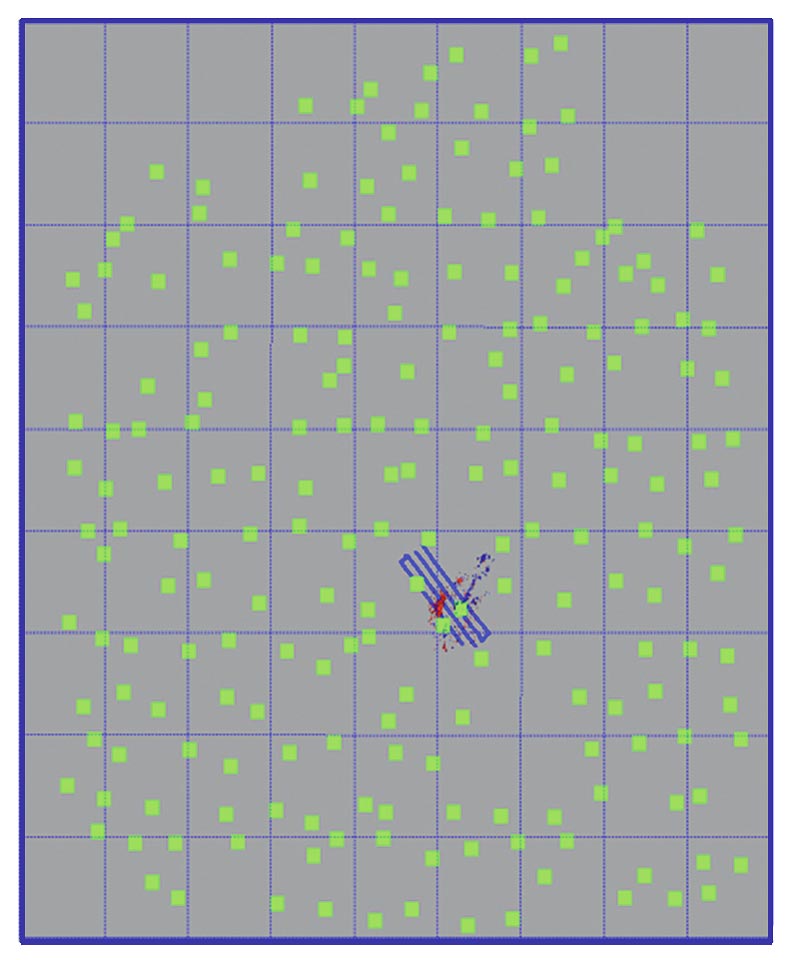
Microseismic data was acquired using MicroSeismic Inc.'s BuriedArray™ technology—a near-surface permanent installation of 618 stations equipped with vertical component geophones distributed over an area of approximately 144 square kilometers (Figure 1).
This passive seismic emission tomography system collected data from the geophone array and imaged it to display how fractures were propagating through the rock during well stimulation. The goal of this study is to identify important structural patterns in the bedrock, especially joints and tectonic faults that reactivate during hydrofracturing stimulation (both are present in the study area).
Fracture and fault events can be differentiated using seismic event statistics. Gutenberg and Richter (1954) first proposed that in a given region, for a given period of time, the number of seismic events of a certain magnitude can be represented by
log N = A – bMs
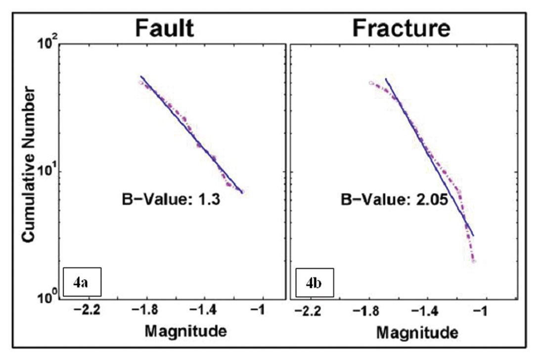
where N is the number of earthquakes with magnitudes in a fixed interval around magnitude Ms, and A and b are variables. Maxwell et al. (2009) and Downie et al. (2010) show that events recorded during hydraulic treatment have a b value of 2, while events associated with fault deformation have a b value of 1. Maxwell et al. (2009) also observed differences in the P- to Swave amplitude ratios that were interpreted as differences in the failure mechanism.
This and other research indicates that b values can be a valuable tool for discriminating between types of fracture propagation. This approach requires a large number of events and can only be performed after the fact. Source mechanism analysis, however, is also capable of providing this information, in real time, for each event. Evaluating b values in combination with event source mechanisms provides another reliable way to differentiate between fault-related and fracture-related microseismic events. Source mechanism inversion techniques can also determine the method of failure experienced by the rock formation, expanding our understanding of the dynamics involved in hydraulic fracturing.
Events in this case study defined two populations based upon the distinct source mechanisms present. Spatial and temporal analysis of frequency magnitude distributions (FMD) allows us to characterize trends useful in assessing the hydraulic treatment efficiency. This information can assist in interpretation of faults in a 3D seismic volume to delineate faults in reservoirs; when used alone it can identify faults of subseismic displacement to further optimize future well placement. Also b values and source mechanisms can help to better define stimulated reservoir volumes (SRV) by indicating the effective level of stimulation. By examining the FMD of event populations we can also determine if a particular type of mechanism is associated with fault activity or the reactivation of natural fractures.
Methodology
Source mechanism inversion of microseismic events can identify failure mechanisms that vary spatially across a treatment. This allows for the separation of microseismic events into populations, giving a more accurate picture of the forces driving the event. We calculate source mechanisms with a least squares inversion of the observed P-wave amplitudes, assuming a point source (Williams-Stroud et al., 2010). The inversion algorithm inverts for full moment (i.e. including the volumetric part of the source mechanism), and double-couple (shear) mechanisms. The moment tensor can be inverted from a point source relationship between observed displacements on vertical component A and moment tensor components Mjk:
A = G3j,k Mjk
where G3j,k are vertical components of the Green's function derivative and Einstein's summation rules apply (Aki and Richard, 1980). This equation can be inverted by either least squares (Sipkin, 1982) or a grid search. The grid search option is possible only for a pure shear source as a non-shear source has an infinite number of possible combinations of Mjk.
We used only P-waves on vertical components for the inversion of the moment tensor, as the aperture and distribution of the array allows a robust solution. The Green's function derivatives of a homogeneous isotropic medium with correction for attenuation can be written as:

For further detail please refer to Williams-Stroud et al. (2010). Source mechanisms presented herein represent the solution that best approximates observed spatial trends of the microseismic events.
The failure mechanisms used to differentiate between events generated by reactivation of natural fractures and events generated by stimulation of a pre-existing fault plane intersecting the wellbore (De La Pena et al., 2011) herein are referred to as fracture and fault events, respectively.
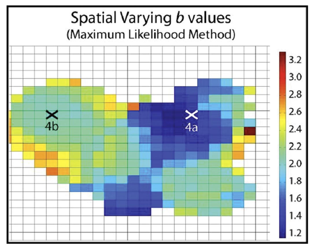
We used Zmap software (Wiemer, 2001) to analyze spatial variation of b values over the areal extent of the microseismic volume. Grid cells are set at 0.001 degrees latitude and longitude (Figure 2). The magnitude of completeness, Mc, which is the lowest magnitude at which all events of that size are detected, was calculated using the maximum curvature method and b values were calculated using the maximum likelihood method (Woessner and Wiemer, 2005). Frequency magnitude distributions are determined by plotting moment magnitude bins of 0.1 against the log of the bin count. The b value was determined by measuring the slope of the histogram for magnitudes above a common Mc of -1.6 for consistency.
Cumulative energy release plots for each mechanism were created by first converting moment magnitude into Joules released per event using the following formula:
logJ = 1.5Mw + 4.8
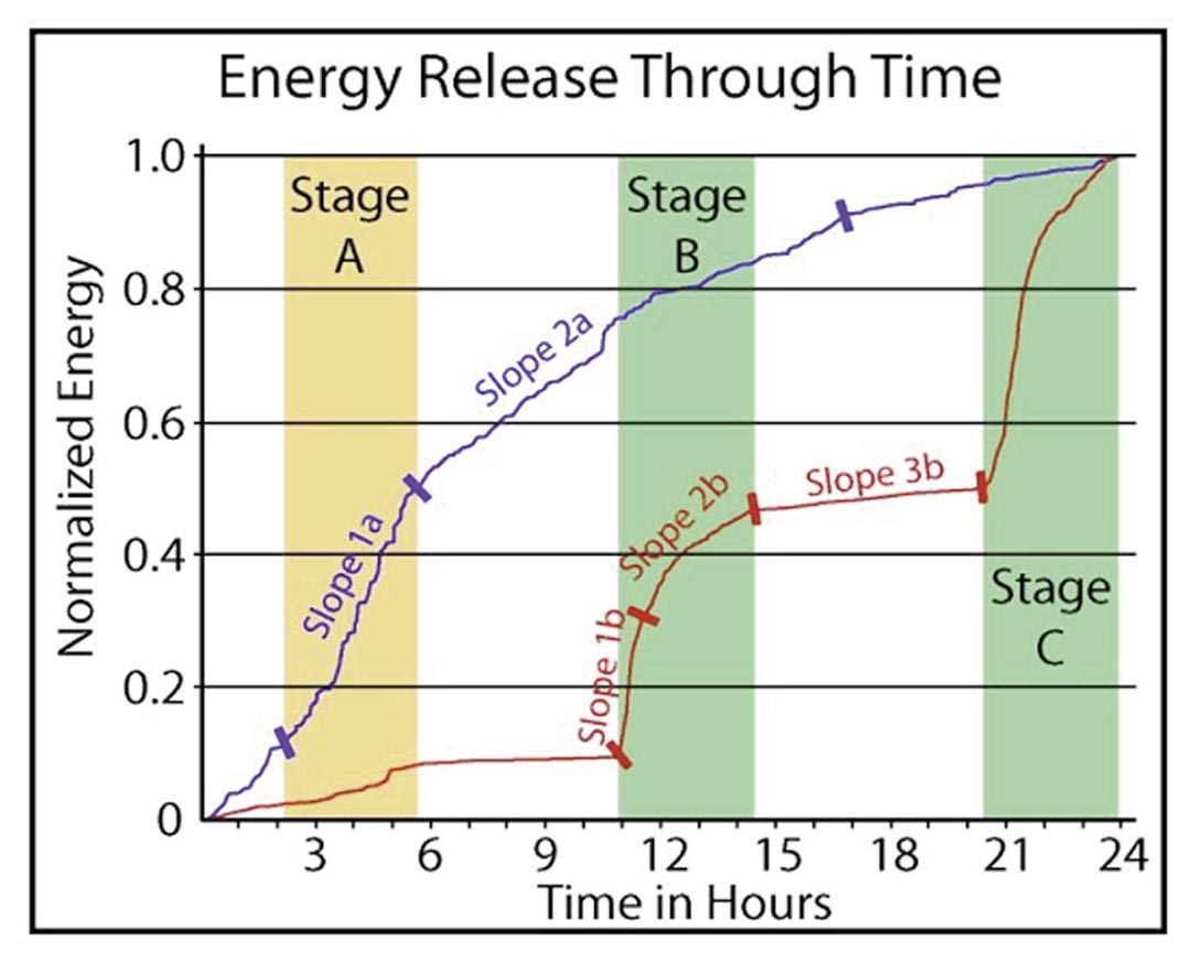
This formula is derived from the equation used by Kanamori and Anderson (1975) to convert moment magnitude to ergs and follows the Gutenberg-Richter energy relationship (Gutenberg and Richter, 1956). Cumulative energy released for a 24-hour period was then summed and normalized to 1 for each population to correct for the disparity in event count and total energy released by events of each mechanism. Slopes were then calculated within chosen time intervals to illustrate the variability in energy release rates of each mechanism (Figure 3).
Case Study
Microseismic data was collected over a three-week period during the stimulation of four horizontal wells in the lower Barnett Shale in Montague County, Texas. The well horizontals are oriented perpendicular to maximum horizontal stress (Heidbach et al., 2009). The treatment was performed in a zippered fashion (western wells treated from south to north and eastern wells in reverse). The data exhibited two dominant source mechanisms during the course of the treatment. Maximum horizontal stress in the region is oriented NE-SW; however natural fractures in the area are oriented WSW-ESE (Waters et. al., 2006).
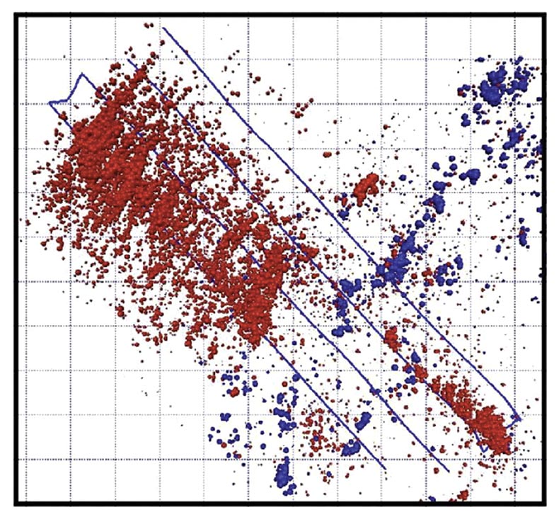
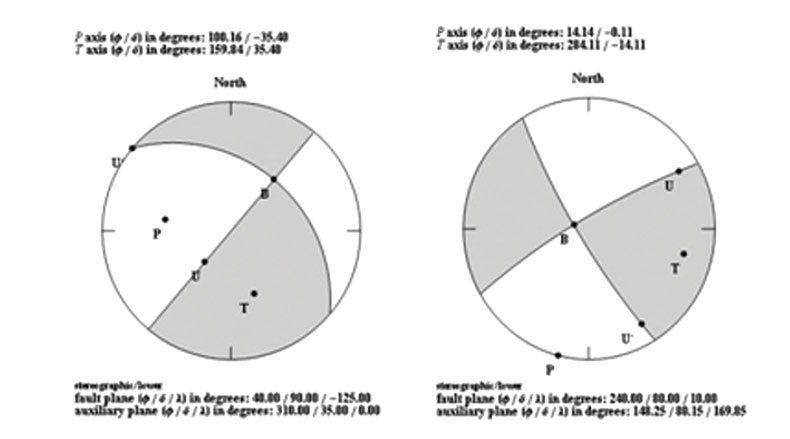
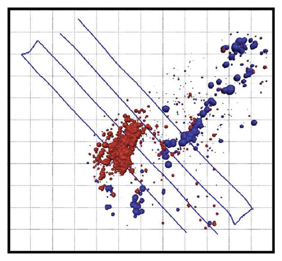
All the wells produced microseismic events with source mechanisms aligned with maximum horizontal stress—oblique slip with left lateral strike slip and normal component down to the north on a vertical plane with a strike of 40-50°. The four wells identify clear trends in microseismic event distribution. Two mechanisms are present: 40/90/-125 in the northwest and 240/80/10 in the southeast. Events with the 240/80/10 source mechanism are concentrated along the blue trend (Figure 4) and were of greater magnitude than other events away from this zone. The blue trend is proposed to be a tectonic fault and also has b values that verify this claim (De La Pena et. al. 2011), making this a good data set to analyze from a real-time standpoint.
Fault versus Fracture Source Mechanism
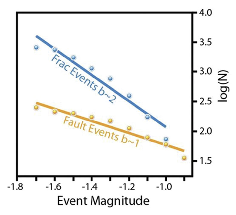
Magnitude values for the microseismic events in the study area were calculated (Figure 5). The data set is comprised of approximately 3,000 events that occurred during the three weeks of treatment. The b values observed for the two different mechanisms support the findings of Downie et al. (2010); i.e. where events that occurred along the fault have a lower slope (b value of 1.0) than events caused by reactivation of joints (b value of 2.2). Downie et al. used fault events that occurred after the treatment to calculate b values while we present events recorded during and after the treatment.
To adapt b values to real time and maintain stability and robustness we used the Tinti & Mulargia equation. When calculating b values, the Gutenberg Richter equation forms the basis of evaluating frequency magnitude distributions with large natural earthquake catalogs. There have been many improvements to the formula since its discovery in order to make more accurate judgments of b values and to take into account sources of error such as binning of magnitudes and temporal variability in minimum catalog magnitudes. For real-time purposes we used the updated equation from Tinti & Mulargia (1987):

Where ΔM is the binning width of the catalog and

Where μ is the average magnitude of the catalog and Mc is the magnitude of completeness or the smallest magnitude at which 100% of events are recorded.
Different source mechanisms within the same treatment suggest a fundamental difference in the character of the events, indicating a fault may be present. Separating the mechanisms creates two independent and growing catalogs. As soon as these catalogs reach a minimum of 50 events in length, they are complete enough to perform a b-value calculation (Figure 6). This occurs 30 minutes from the initial event for each catalog. Once both catalogs reach 50 events, the b value for the catalog is recalculated using an expanding window, such that each new event is added to the appropriate catalog and the b value is recalculated for the whole data set.
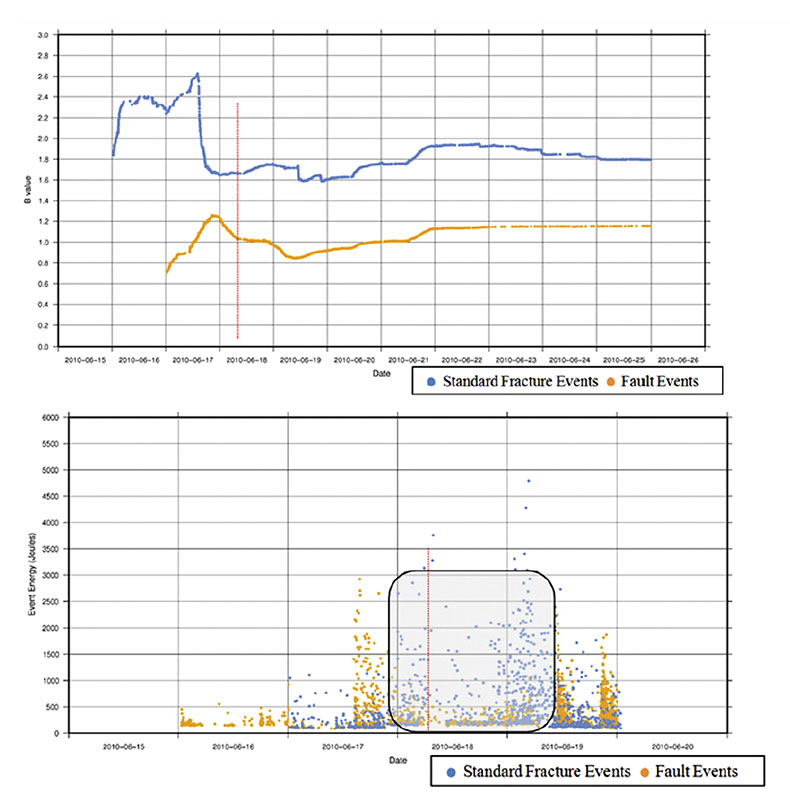
The minimum magnitude of completeness is recalculated at each step by maximum curvature; however each mechanism showed a unique magnitude of completeness over the entirety of each data set with the 040/90/-125 mechanism showing a magnitude of completeness of -1.7 and the 240/80/10 mechanism showing a magnitude of completeness of -1.8. In order to identify faults in real-time operations, we would need to see the b values for one of the two source mechanism reach a stable trend of ~2. This means that as we watch the curve in real time a b value signature stabilizing around a value of 1 is a signal that this mechanism is associated with faulting.
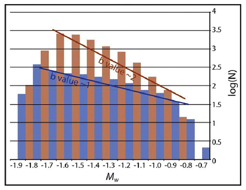
Examining the FMD of events can give us more information about how the rock formation breaks and what external factors may be involved. Maxwell et al. (2009) and Downie et al. (2010) differentiate fault movement from fracture stimulation by comparing the slope (b value) on FMD plots for different populations of events. Figure 7 shows two different b value populations— slopes of ~2 for fracture events and ~1 for fault events (De La Pena et al., 2011).
Fault events on average release a greater amount of energy and have a greater maximum magnitude when compared to fracture events; however, there are significantly fewer fault events than fracture events within this dataset. This is a result of the relatively small but linear area affected by the fault relative to the broad and well-distributed fracture development.
The spatial variation in b values (Figure 2) indicates the relative presence of fault activity vs. fracture activity and largely mirrors the event distribution seen in Figure 4. Lower b values are concentrated where the fault crosses the wellbores whereas higher b values indicate typical fracture event generation. The spatial distribution of b values in Figure 2 shows the variation between areas of effectively stimulated reservoir relative to areas that may not have been so effectively stimulated. The highest b values located near the outer edges of the treated area are anomalously high due to an insufficient event population per cell. FMD plots for individual cells (Figure 8) within Figure 2 are in agreement with our b values for the total population of fault and fracture events.
Timing and Rates of Energy Release
Microseismicity generated by hydraulic pumping within a formation with low differential stress should theoretically be coincident with the time of pumping—i.e.when fluid and proppant are forcibly added to the formaton. Similarly, we would expect high-stress areas of the formation to generate microseismicity during pumping and also between pumping intervals when accumulated stress is released. Using microseismic events generated during one 24-hour period (Figure 9), we show that fracture generated microseismicity is largely isolated to a restricted period of pumping time whereas fault events are distributed over a much longer period of time (Figure 3).
Looking at Table 1 and Figure 3, fault energy release during pumping occurs at a moderate rate (slope 1a) followed by a lower rate (slope 2a) that approximates an exponential decline curve. In contrast, we see that hydraulically stimulated natural fractures release microseismic energy at a very high rate initially (slope 1b), followed by a lesser energy release rate (slope 2b) and near inactivity between stages (slope 3b).
| Failure Type | Slope | Slope Value J/s |
|---|---|---|
| Table 1. Slope Values | ||
| Fault | 1a | 9.0 |
| 2a | 3.0 | |
| Fracture | 1b | 42.2 |
| 2b | 7.8 | |
| 3b | 0.8 | |
Therefore we find that microseismic energy released by reactivated fractures is cyclical, predictable, and directly controlled by pumping (slopes 1b, 2b). Between pumping some fracture microseismicity is present, likely due to metastable energy release as the local stress state moves toward equilibrium. The energy release rate of the fault slope 1a is much less than that of the fracture slope 1b, both of which are generated during pumping. The large difference is likely because the fault zone can accept a larger volume of fluids per Joule of microseismic energy released per unit of time. Slope 2a represents the gradual release of energy along the fault plane, which continues for the remainder of the 24 hour time period. Over the continuing course of the stimulation, total energy released in fault affected stages is reduced relative to fracture only stages.
Conclusions
The use of source mechanism inversion to differentiate between rock failure mechanisms combined with b value analysis and energy release rates can give insight into the local stress of the reservoir and confirm or deny the presence of stressed tectonic faults. The type of mechanism that is most mechanically dependent upon pumping can be assumed to be the desired fracture type because it is related to events that are evenly distributed throughout the reservoir rather than being related to large fault-like features. If there is a mechanism that exhibits energy release rates that are not dependent upon the pumping schedule it is likely to be a pre-existing feature that is optimally oriented to fail in the current stress field. These assumptions are validated by b value analysis of the event populations and spatial trends of the microseismic events. Spatial b value distribution maps are a potentially powerful tool to better estimate what portions of the reservoir are successfully stimulated.
This information can be used to better define stimulated reservoir volumes by separating mechanically independent (fault related) microseismicity from the total interpreted stimulated volume to more accurately represent the volume of rock that fractured under desired conditions. The presence of relatively large magnitude events after the fracture stage is completed can also indicate stimulation of a fault plane. If this data is available to an operator during hydraulic stimulation it can indicate whether a fault is stimulated, allowing the operator to make a decision to alter the pumping schedule or continue treatment on an interval away from the fault plane, thereby optimizing costs, use of materials, time, and treatment efficiency.
On this treatment to proposed fault hits full activation at ~6:00 am on the 19th , while positive id of a fault signature occurs 24 hours earlier . In this case we define full activation as the feature realizing its’ full length. We see a positive id in all three indicators well in advance, before it is able to reach full activation and waste time and resources. By skipping past the fault feature before continuing the treatment, its’ potential effect on the treatment and production of the well can be minimized. Here this would mean saving three stages worth of fracing materials, not to mention 24 hours of work that will not be contributing to the effective stimulation of the well.
Discussion
Engineers require reliable information during hydraulic treatment to make knowledgeable decisions and optimize resources. Microseismic monitoring is an effective tool in the development of shale plays and a primary method for understanding the geomechanical properties of the reservoir. The use of source mechanism inversion, combined with b value analysis and energy release rates, to differentiate between rock failure mechanisms (faults versus joints) provides insight into the local stress of the reservoir and confirm or deny the presence of stressed tectonic faults. Spatial b value distribution maps of microseismic events are potentially powerful tools to better estimate what portions of the reservoir are successfully stimulated; the more desired fracture-type mechanism is more evenly distributed throughout the reservoir compared to larger, fault-like features.
This information can be used to better define stimulated reservoir volumes by separating mechanically independent (faultrelated) microseismicity from the total interpreted stimulated volume to more accurately represent the volume of rock that fractured under desired conditions. The presence of relatively large magnitude events after the fracture stage is completed can also indicate stimulation of a fault plane. If this data is available to an operator during hydraulic stimulation it can indicate whether a fault is stimulated, allowing the operator to make a decision to alter the pumping schedule or continue treatment on an interval away from the fault plane, thereby optimizing costs, use of materials, time, and treatment efficiency.
In addition to optimizing reservoir stimulation and production, microseismic monitoring has other benefits as well. It can provide the factual evidence necessary to counter environmental objections to hydraulic fracturing; for example, the threat to aquifers or public water supplies. Other applications include reservoir monitoring and earthquake monitoring. Microseismic technologies can also be used to check cyclic steam injection processes in heavy oil production and the integrity of underground salt domes that store hydrocarbons and chemicals.

Related Reading


Join the Conversation
Interested in starting, or contributing to a conversation about an article or issue of the RECORDER? Join our CSEG LinkedIn Group.
Share This Article