Integrated fluid-flow, geomechanic and seismic modelling for reservoir characterisation

1. Introduction

Solutions to large number of problems facing the petroleum industry during exploration, appraisal and production require integration of knowledge and workflows from a range of disciplines including geology, petroleum engineering, geomechanics, rock physics, petro-physics and geophysics; in the future CO₂ storage projects will also require such an integrated approach. Over the past few decades 4D seismic and microseismic monitoring have been used to image areas of bypassed oil, the geometry and nature of reservoir flow compartments, regions of high stress and hydraulic fracture development, but with varying degrees of success. Whether these surveys are successful is heavily influenced by the overall complexity of the reservoir and surrounding strata (e.g., structural, sedimentelogical and mechanical heterogeneity, etc.), which can alter the relationship between seismic velocities and the fluid-flow and rock physical properties as well as the stress and strain fields. Thus, to improve interpretation of 4D seismics and microseismicity for prediction of long-term well stability, evaluation of the risk of sea floor subsidence, and prediction of long-term reservoir flow behaviour requires an integrated approach.

The main goal of the recently completed multidisciplinary research consortium Integrated Petroleum Engineering, Geomechanics and Geophysics (IPEGG) was to develop and apply coupled fluid-flow and geomechanical simulation and integrate with seismic modeling to help predict reservoir behaviour. To achieve this, the finite-element (FE) geomechanical solver ELFEN™ (Rockfield Software) was used as the central engine of the integrated package using its preprocessing, geomechanical solver and post-processing facilities to manage the workflow. As such, the primary focus of the geophysical component of IPEGG has been to interface and use as much information as possible from the coupled fluidflow and geomechanical simulation. Specifically, a suite of rock physics models was incorporated to advance seismic model building capacity and improve seismic attribute prediction.

Segura et al. (in press) provide an extensive study on the influence of reservoir geometry and material properties on stress path during production using coupled fluid-flow and geomechanical simulation. Using poroelastic constitutive material behaviour, Segura et al. (in press) observed that the stress arching effect is significant in low aspect ratio reservoirs that are soft compared to the surrounding rock. Under such circumstances, the total stress does not change significantly within the reservoir and so stress evolution occurs primarily in the overburden and side-burden. Furthermore, stiff reservoirs do not display any stress arching regardless of the geometry. Stress anisotropy reduces with reduction in the stiffness of the bounding material (e.g., Young’s modulus), and this is especially true for small reservoirs. However, when the dimensions extend in one or two lateral directions the reservoir deforms uniaxially and the horizontal stresses are controlled by the reservoir Poisson’s ratio.

This paper presents a summary of the achievements made with the IPEGG project, with focus on the seismic developments and applications of the integrated flow-geomechanics and seismic modeling. We present the integrated workflow discussing briefly the geomechanical finite-element grid generation, geomechanical constitutive model, coupling fluid-flow and geomechanical methodologies, rock physics modeling, and building seismic models. We demonstrate the integrated workflow using three cases studies; a model of a simple graben structure, a conceptual model of the Weyburn CO₂ storage pilot study and a sub-volume of the Valhall reservoir in the North Sea. We conclude with project highlights and future directions.

2. Integrated workflow

To develop the integrated workflow, the project addressed the following technological aspects:

Generation of finite-element (FE) grids from geological models:

The preliminary stage in generating a geomechanical model is to generate FE meshes based on geological models of the reservoir, over-, under- and side-burden. Such a model must be ‘water-tight’, that is to say that there must be no gaps in the mesh and each node must be connected to surrounding nodes. Faults and other subsurface discontinuities present the biggest challenge in this respect, and they must be handled carefully when exported from a geological model (such as PetrelTM or GoCAD™) into an FE simulator. We have expanded our FE model pre-processor functionalities to handle more sophisticated grids describing real horizons and fault geometries using a specific tool to import the geometry defined by standard subsurface model generators. Once imported, the geometry can be meshed using structured or unstructured meshes, assigning different mesh sizes to different volumes, or assigning a more dense mesh in specific zones, among other functionalities.

Population of FE models with geomechanical properties:

Once a mesh has been generated, each node must be populated with mechanical properties – for elastic deformation the Young’s modulus, Poisson’s ratio, porosity and density must be specified. Young’s modulus and Poisson’s ratio need not be isotropic. For inelastic constitutive models additional parameters such as Unconfined Compressive Strength (UCS), angle of internal friction, tensile strength, and critical compaction pressure must also be defined. Any faults must be given values for cohesive strength and friction coefficient. The ELFEN™ FE model pre-processing facility contains a large material library for assignment to each material layer defining the reservoir as well as over-, under-, and side-burden. It is based on a modified version of the Cam-Clay model specifically developed for modelling of soft rocks (Crook et al. 2002). The program has also some utilities to adjust the SR3 (isotropic or orthotropic) or the Mohr Coulomb model parameters against experimental data from uniaxial, triaxial and hydrostatic laboratory tests.

Coupling methodologies:

Geomechanical deformation in and around a reservoir is driven by pore-pressure changes in the reservoir induced by production and/or injection activities. Therefore, geomechanical models should use accurate fluid-flow simulations to apply a load to the reservoir. The simplest fluid-flow/geomechanical simulation coupling method is the ‘one-way coupling’ method, where porepressures are passed from a history-matched fluid-flow simulation to a geomechanical simulator at regular time-steps.

However, geomechanical deformation, if it alters porosity and permeability through compaction of a producing reservoir for instance, can affect fluid-flow in the reservoir, so a reciprocal coupling is required, where changes in porosity computed by the geomechanical simulation are returned to update the flow simulation. A number of methods exist to couple fluid-flow and geomechanical models (e.g., Settari & Moutts 1998; Dean et al. 2003). Conceptually, it is possibly to solve the equations for fluid-flow and deformation simultaneously within the same simulator. This ‘fully-coupled’ method would be the most numerically accurate. However, the industry has expended much effort in the last 30 or so years to develop fluid-flow simulators capable of accurately solving complex multi-phase flow simulators. Thus if we can use these commercial simulators to provide fluid-flow models on which to base geomechanical simulation, without extensive modification, then this would be extremely advantageous.

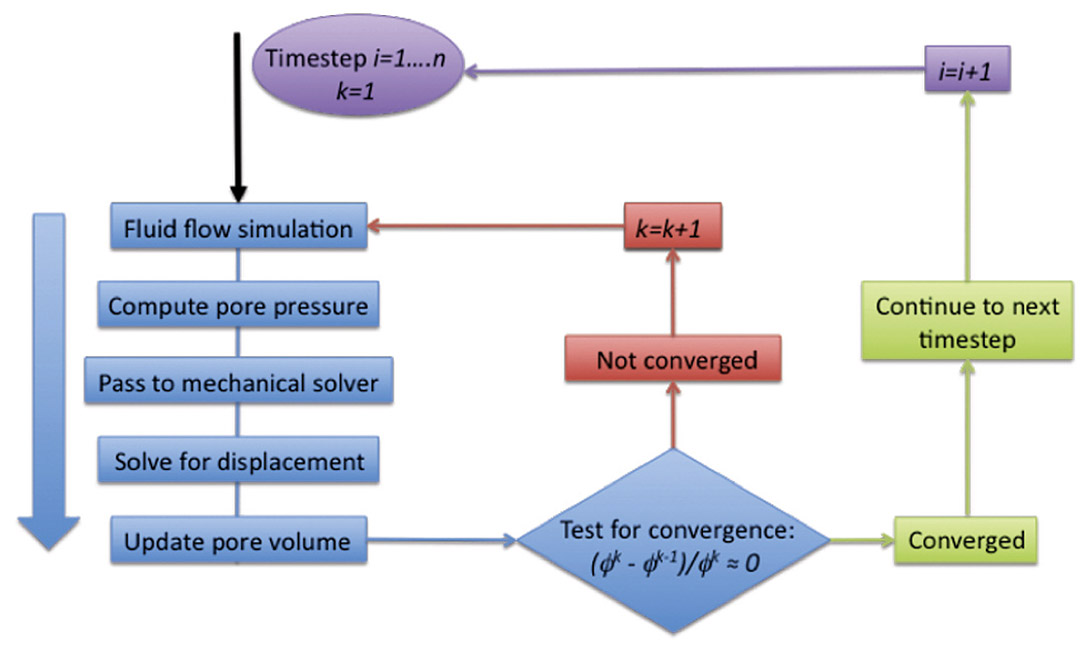
There are two methods available to couple separate fluid-flow and geomechanical simulators together in a bi-directional manner: explicit coupling and iterative coupling (Dean et al., 2003). For the explicit coupling method, the fluid-flow and geomechanical simulators are run in parallel, as per the one-way coupling method, except that at given time-steps when porepressures are passed to the mechanical simulation, changes in fluid-flow parameters are returned to update the flow simulation. The iterative method is similar to the explicit method, except for at each time-step the fluid-flow and deformation are solved in an iterative manner, with data passed back and forth between the simulations until a stable solution is found. This is illustrated in Figure 1. At each time-step the fluid-flow simulator computes the pore-pressure and fluid properties. These are passed to the geomechanical simulator to compute deformation. The mechanical solver computes changes in porosity, which is returned to the flow simulation to recomputed pore pressures using the updated pore volumes. This iterative process, passing pore pressures and pore volumes between the mechanical and flow simulators, is iterated until a stable value for porosity (and a corresponding value for pore pressure) is reached, at which point the simulation moves to the subsequent time-step.

Comparison between the coupling methods suggest that the iterative method provides the best combination of the possibility of using existing industry flow simulations; computational efficiency; and accuracy of results that match those provided by fully coupled simulations (e.g., Longuemare et al., 2002). Alternatively, if the time integration of geomechanical field is performed in an explicit fashon, high frequency explicit coupling between the geomechanical and flow fields and provide similar accuracy and efficiency to iterative coupling for many applications. Such coupling methods can be achieved by writing data to file at each computational step to be read by the different simulators. However much computational efficiency can be gained if the data is passed between simulators using message passing interface process.

Rock physics modelling:

To predict the seismic response based on the results of coupled fluid-flow/geomechanical simulation, rock physics models are required that map changes in fluid saturation, pore pressure, and effective stresses into seismic stiffness. To describe the full seismic response, in terms of P-and S-wave propagation in arbitrary directions through an anisotropic medium, such a model should use as its basis the 21 components of the full dynamic stiffness tensor (dynamic here refers to the length- and time-scale of a seismic wave: low strain magnitude, high strain rate). The workflow used to build the dynamic elastic model is based on constructing an aggregate elasticity (Angus et al., 2007) starting from the micro-scale (e.g., intrinsic anisotropy) and working up to the macro-scale (field-scale fractures). Such a model should account for intrinsic rock properties and microstructural fabrics (e.g., Kendall et al., 2007; Hall et al., 2008), stress-dependent seismic velocities (e.g., Verdon et al., 2008), and fluid substitution effects either at low frequency (Gassmann, 1951) or including dispersive effects induced by squirt-flow (Chapman, 2003). The influence of coherent fracture sets is modelled using Hudson et al. (1996) and Schoenberg & Sayers (1995).

During geomechanical simulation, a range of physical properties needed to model the dynamic stiffness are defined or computed at each node in the simulation. For example, the static stiffness, where static refers to the time- and length-scales for geomechanical deformation (high strain magnitude, low strain rate) is often observed empirically to calibrate with dynamic stiffness (e.g., Olsen et al., 2008); the porosity is required to solve Gassmann’s equation for fluid substitution; the effective stress tensor is required to compute the effects of stress on dynamic stiffness (non-linear elasticity); and the density is required along with the dynamic stiffness to compute seismic velocities. There are also parameters, such as the microcrack properties needed to compute stress-dependant stiffness (see below), that are not involved in any geomechanical simulations and therefore must be defined based on prior knowledge of the rocks being measured.

The geomechanical simulation outputs the appropriate parameters on a node-by-node basis. The static stiffness is used as a starting point for computing the dynamic stiffness, as we assume that the static stiffness is scaled to the dynamic. This basis is used to incorporate the effects of stress dependent stiffness using the microstructural approach of Verdon et al., (2008). Once the stressdependent effects have been incorporated, the effects of fluid substitution are computed using either the low frequency Gassmann equation or the frequency-dependent, attenuative model of Chapman (2003).

We adopted the micro-structural model of Verdon et al. (2008) to model nonlinear elasticity because it represents a conceptually attractive approach to describe the stress dependence of seismic velocity and anisotropy. This model assumes that a fraction of the total porosity of the rock can be considered compliant. Although negligible in volume, the compliance of these features, sometimes referred to as microcracks, dominates the nonlinear stiffness response. As stresses increase, these features are forced closed, increasing the seismic velocity and reducing the stress-sensitivity, matching the nonlinear response that is empirically observed.

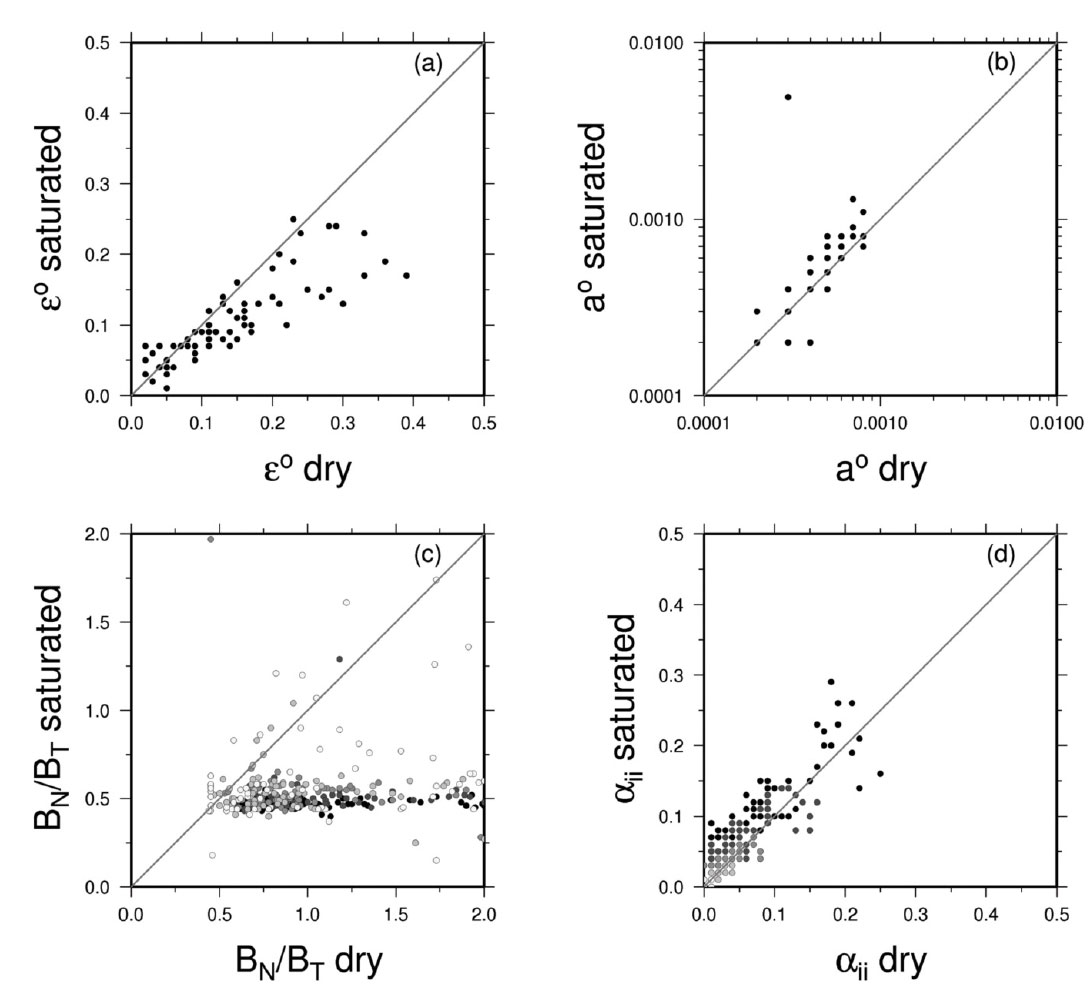
The necessary input parameters for the nonlinear stiffness model are the background elasticity, triaxial stress tensor, and the initial microcrack density and aspect ratios (see Verdon et al. 2008). The initial microcrack density and aspect ratio are defined independently from the geomechanical simulation. Verdon et al. (2008), Angus et al. (2009; in review) have calibrated these parameters using over 200 sets of ultrasonic velocity versus stress data measured on dry and saturated core samples from the literature. Figure 2 demonstrates some results of calibrating the rock physics models on dry and brine saturated core data (see Angus et al., 2009, for discussion of calibration technique).

The static stiffness used in the geomechanical model, once scaled appropriately, can be considered to represent the dynamic stiffness at the initial reservoir stress conditions. This, along with the microcrack properties taken from core measurements, provide enough information to initialise the stress-sensitive rock physics model, allowing the effects of stress change during production to be incorporated into the seismic response.

The elastic models incorporate a range of rock physics models, the seismic models can be isotropic or anisotropic as well as acoustic, elastic or visco-elastic. The choice of model depends on what attributes are sought as well as what type of seismic modelling algorithm is to be used (e.g., anisotropic ray tracing, full-waveform isotropic or acoustic finite-difference simulation, elastic anisotropic one-way wave equation). Given that the elastic model can be generally anisotropic and heterogeneous, there is a large scope of seismic attributes that can be modeled, such as Pand S-wave velocity changes (absolute, horizontal and vertical), Thomsen parameters, and general seismic anisotropy (e.g., shear-wave anisotropy).

Microseismic Predictions:

Another important observable manifestation of geomechanical deformation that can be used to link with geophysics is microseismic activity. For elastic models, regions of high shear stress should correspond with regions at an increased risk of microseismicity. When mechanical simulations include brittle and plastic behaviour in their constitutive models, this can be used as a direct indicator of microseismic activity. There remains a degree of uncertainty as to the best method to make predictions about microseismic activity based on geomechanical models.

A key difficulty is the difference in scale between field geomechanical models and the length-scale of a microseismic event: typically elements in a mechanical model might have dimensions of the order of 50m. A typical microseismic event is produced by slip on a feature of meter to sub-meter scale. For this reason a coupled fluid-flow and discrete element (CFD-DEM) approach also offers strong potential in predicting microseismicity (e.g., Hazzard et al., 2002). Since CFD-DEM is a particle based formulation (i.e., it does not assume continuum, unlike FE models) it provides a natural representation of fracturing. However, due to computational requirements it is limited to much smaller volumes than provided by FE models.

We have developed two parallel methods to make predictions about microseismicity on a reservoir scale based on mechanical models. The first approach is to consider the evolution of deviatoric stress with respect to the Mohr-Coulomb failure envelope. This can be formalised using the fracture potential term, f^p (e.g., Verdon et al., 2011), which describes the ratio of the in situ deviatoric stress to the critical stress required for failure on an optimally oriented surface: f^p=q/q^crit. A higher value for fp corresponds to a higher risk of microseismicity for the node in question. Alternatively, the Coulomb failure stress change or Coulomb yield stress change (e.g., Soltanzadeh & Hawkes, 2008; Rozhko, 2010) can be adopted.

The second method tracks matrix failure during the geomechanical simulation. This microseismic modeling approach allows for a continuous monitoring of the temporal and spatial distribution of seismicity (see Angus et al., 2010). In the matrix failure approach, the geomechanical solver internally tracks regions undergoing yield and for each failure, the stress tensor, pore pressure and elastic tensor are output to a microseismic file. Since ELFEN™ is an FE based geomechanical solver, the microseismic predictions are limited by the continuum formulation (i.e., not localized). Clearly this is an oversimplification of the physics, but it does provide a first-order estimate of regions within the model that might generate seismicity and potential the type of failure (tensile, shear or shear-enhanced compaction).

3. Case Examples

Having outlined our modelling workflow, we will now demonstrate it in practice for several examples, working up in complexity from a purely synthetic example, through a simple approximation of a real field, to a full-field simulation.

Two fault model:

The first model we consider is a graben-style reservoir, consisting of three compartments separated by two normal faults. To investigate the possibilities of using geophysical observations to detect compartmentalisation, we have created two versions of this model – where the faults are sealing and where they do not seal. Angus et al., (2008) presented initial results from the coupled flow-geomechanical simulations to show the effect of fault transmissibility on various seismic attributes. For the high transmissibility example, travel-time anomalies for both the overburden and reservoir are observed over the lateral extent of the reservoir and indicate that the two normal faults may act as a stress guide. As fault transmissibility is reduced, the traveltime anomalies become more localized. Shear–wave splitting shows similar patterns.

Figure 3 displays seismic P-wave evolution from production of a graben style reservoir characterized by two normal faults subdividing a sandstone reservoir into three compartments (see Angus et al., 2010). For this particular model, the production well is vertical located at approximately x=1000 m and y=1500 m, and the faults are sealing (i.e., no fluid-flow across the fault). In this figure, the reservoir is located at approximately 3000 m depth and laterally between 0 and 7000 m in x and 0 and 3000 m in y (see thin red region at depth). Shown are the contoured average P-wave velocity for the initial base state, the evolved P-wave velocity after approximately 10 years of production and the change in P-wave velocity. In this example, a decrease in velocity is observed in the over- and under-burden and an increase in velocity within the reservoir and in the side-burden. In the near surface, there is an increase in velocity above the producing reservoir. Though it should be stressed that the rock physics model parameters have only been calibrated for rock at or near reservoir depths and so the model is likely over stress sensitive near the surface. This stresses the importance of measuring near surface rock properties for better prediction of subsidence and related risks. A recent literature search suggests that this type of data is lacking.

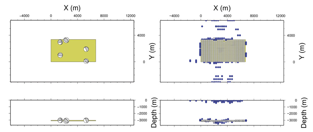
Figure 4 shows the results of modeling source mechanisms (double-couple solution in this case) as well as spatial and temporal event distribution. In this example, the faults are nonsealing (i.e., do not act as a barrier to flow) and so production of fluid occurs over the whole reservoir (as opposed to only the lefthand compartment in Figure 3). The sandstone reservoir fails under a shear-enhanced compaction type mechanism where as event outside the reservoir fail under shear. In this case, the sandstone graben structure acts as an extensive reservoir and hence compaction within the reservoir impacts the stress field significantly into the near surface and leads to small shear-type seismicity. Angus et al. (2010) show, that for this reservoir geometry, fault movement as well as fluid extraction can influence the spatial, temporal and scalar moment of microseismicity. For nonsealing faults, failure occurs within and surrounding all reservoir compartments and significant distribution located near the surface of the overburden. Movement of faults leads to increase in shear-enhanced compaction events within the reservoir and shear events located within the side-burden adjacent to the fault. The moment magnitude distributions of shear events show low values near the surface, moderate values near the faults and high values along the reservoir boundary. Overall, the results from the study indicate that it may be possible to identify compartment boundaries based on the results of microseismic monitoring. This is potentially an important result given the uncertainty of existing methods to predict the extent of fault compartmentalization and particularly the position of compartment boundaries (Fisher & Jolley, 2007).

Simple model of the Weyburn CCS-EOR reservoir:

Our second model is a simplified representation of CO₂ injection for CCS/EOR at Weyburn. The model, described in more detail in Verdon et al. (2011), has been developed to aid interpretation of microseismicity detected during injection (Verdon et al., 2010). The Weyburn reservoir is laterally extensive and relatively flat, so has been modelled using flat layers and a rectangular grid. The reservoir is a 40m thick carbonate unit, over and underlain by evaporite sealing layers. An overlying shale layer provides a secondary seal. The reservoir is being produced through horizontal wells trending NE-SW, and in the region of interest CO₂ is injected through vertical wells. A fluid flow model was developed to approximate this geometry of producers and injectors. The modelled locations of vertical injectors and horizontal producers can be seen in Figures 5a-c. After an extended period of production (Weyburn has been in production since 1955) we simulated 1 year of CO₂ storage, injecting at a pressure of 20MPa through a vertical injection well while continuing to produce oil through horizontal producers on either side of the injection site.

This fluid-flow simulation provided the loading with which to compute stress changes inside and around the reservoir. We are most interested in what the geomechanical model predicts in terms of microseismicity. To generate predictions about microseismic activity we use the fracture potential method to identify regions of the reservoir and overburden that are experiencing elevated shear stresses with respect to critical shear stress, and therefore are assumed to be most prone to seismic activity. Maps of percentage change in fracture potential in the reservoir and cap-rock during the injection phase are shown in Figure 5a,b.

Conventional ideas about injection- induced seismicity suggest that pore pressure increases around an injection well should reduce effective normal stresses, increasing the probability of shear and/or tensile failure (Shapiro 2008, and references therein), meaning that microseismicity should initiate around the injection well before migrating radially outwards. However, our geomechanical models indicate that in this case, the stress evolution induced by injection, although it does reduce the effective normal stress, also serves to reduce the effective shear stress, so the fracture potential is in fact reduced. In contrast, in the overburden above the production wells there is little change in effective normal stress, yet an increase in the shear stress, serving to increase the fracture potential in this region.

Our geomechanical model implies that we should expect microseismicity to be located around the production wells and in the overburden at Weyburn, not around the injection well. Details about the observed microseismicity can be found in Maxwell et al. (2004), White (2009), and Verdon et al. (2010) – we have found that microseismic events are indeed located in the reservoir and in the overburden around the production wells (Figure 5d), and not around the injection well, as predicted by the geomechanical model. We have also used the Verdon et al., (2008) rock physics model to predict seismic anisotropy in the overburden. A map of modelled shear-wave splitting is plotted in Figure 5c. The predictions made – that above the injection well the fast direction should be perpendicular to the horizontal well trajectories, is matched by anisotropy observations made by measuring splitting of shear waves produced by the microseismic events (Verdon et al. 2011; Verdon & Kendall 2011).

Full Field Case Study:

Probably the most challenging aspect currently is full-field reservoir simulation, which requires realistic geomechanical properties, development of water-tight meshing, production history matching and significant computational resources. There have been some recent successes in applying coupled fluid-flow and geomechanical simulation with seismic modelling to predict 4D seismic field observations. Herwanger et al. (2011) applied the integrated flow-geomechanics-seismic developed by WesternGeco and Schlumberger at South Arne, Danish North Sea to quantify reservoir depletion from 4D seismic surveys. Zhang et al. (2011) model depletion related microseismicity at Valhall based on monitoring the inelastic shear strain.

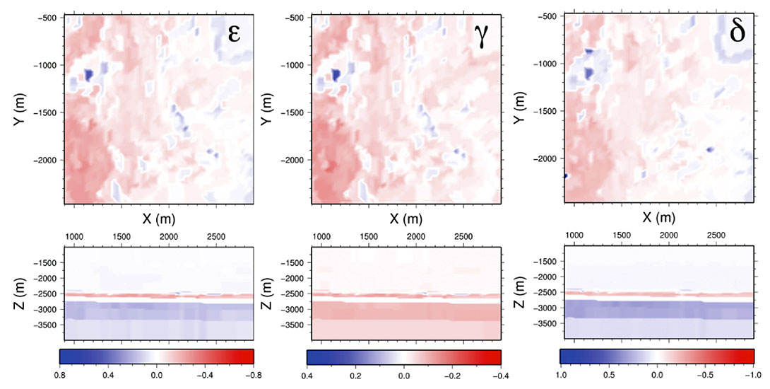
We have generated a geomechanical simulation for a portion of the Valhall Field using a geological model to generate lithological surfaces and the FE mesh, and a history-matched fluid-flow simulation. We have used this model, in combination with our rock physics model, to predict changes in the Thomsen anisotropy parameters, shown in Figure 6. In general, the reservoir displays negative changes (red) in Thomsen parameters, which is expected for a compacting reservoir. However, there are regions showing significant positive changes (blue) in Thomsen parameters indicating extensional regions within the reservoir possibly related to stress arching due to compartmentalisation.

4. Conclusions

The key achievements of the IPEGG consortium were successful coupling of ELFEN™ with several reservoir simulation models and integration with seismic forward modelling for seismic attributes. The integrated workflow has been used to assess the controls on reservoir stress path, use of microseismicity and 4D seismic for detecting reservoir compartmentalization as well as top seal integrity, and the need for coupled fluid-flow and geomechanical production simulation modelling.

There are still significant knowledge caps that need to be improved to reduce the uncertainty of full-field predictions. Specifically, calibration of the models is potentially the most important area for future research (e.g., Settari et al. 2009). With so many uncertainties, it is important that attempts are made to compare predictions from these coupled models with real field data (e.g. surface subsidence, microseismicity, 4D seismic, measured stress paths, production rates etc.). For example, Kristiansen & Plischke (2010) use full field coupled flow-geomechanical modelling incorporating water weakening and re-pressurization to compare predictions of reservoir compaction and surface subsidence with observations at Valhall. Utilizing the integrated workflow developed by IPEGG, there is now a strong potential in constraining geomechanical models with more quantitative comparisons to 4D seismic and microsesimicity. From our experience in other areas (e.g. fault seal analysis), calibration of the models is probably best achieved through field specific case studies with asset teams to encourage maximum buy-in from those working on the specific assets.