Isostasy and Gravity Modelling: Integrating Potential Field Data in Interpretation Workflows

1. Introduction

Potential field data, namely gravity and magnetic data, provide a relatively low cost means of mapping regional geological trends and structures. Magnetic data are typically of most value in regions where igneous and metamorphic rocks are common and they have proved particularly vital for understanding the structure and age of continental and oceanic crust. Indeed, the recognition by Vine and Matthews (1963) of magnetic ‘striping’ in the world’s ocean basins provided the final proof of plate tectonic theory. Gravity data are more commonly used in oil and gas exploration as they can be used to establish the limits and structure of sedimentary basins and predict structural trends. Satellite altimetry data released in the 1980s and 1990s have been processed to provide gravity data for all marine basins with no cost to the end-user (Sandwell and Smith, 1997), and although these data have their limitations they are a valuable reconnaissance tool.

Gravity data are typically forward modelled or inverted to provide a means of interpreting the data, however, modelling and processing methodologies vary depending on the environment, type of target or objective. This paper discusses a number of assumptions that are important to consider when undertaking gravity modelling studies. The paper also includes a short case study that is focused largely on generating isostatic anomaly data in a rift margin setting utilizing seismic reflection data as a geometric constraint and magnetic anomaly data as further validation of physical properties indicated from gravity modelling.

2. Gravity Data

Gravity data are typically reported as ‘anomaly values’ that are calculated from raw measurements. A correction must be applied to raw data for latitude (as the Earth is not a perfect sphere the theoretical gravitational field strength is not equal at all locations – in fact it is greatest at the poles as the Earth roughly approximates an oblate spheroid that has a maximum diameter at the Equator and the poles are therefore closer to the centre of mass of the Earth). Additional corrections are required if data is acquired aboard a moving vessel, such as a ship or plane. The degree of subsequent processing depends, largely, on scale and environment.

A free-air correction is generally applied to data that is not acquired at sea level, this correction is applied to compensate for the elevation at which a measurement is made (because the strength of the gravitational field of a mass is proportional to the inverse square of the distance from the centre of mass of the body). Following this free-air correction we refer to the data as free-air anomaly (FAA) data. In marine environments data are typically not processed any further, however, in land settings a subsequent correction, the Bouguer correction, is typically applied.

The Bouguer correction, accounts for the density of material between the measurement surface and mean sea level (or the geoid). This can be done most simply by assuming that the topographic elevation at the measurement point can be approximated by an infinite slab of a given reference density. The Bouguer correction can be refined by applying a terrain correction, which accounts for the obvious failings of assuming an infinite slab and corrects the FAA data using topographic data surrounding the measurement station. The advent of widely available digital elevation models allow this correction to be implementedhas made implementation of 3D terrain corrections far more easilysimpler than in the past where painstaking manual “ring” calculations were required for each measurement station.

If a Bouguer correction is not applied on land, then the FAA data isare is typically strongly correlated to topography and may be of limited interpretative value. However, a major limitation of the Bouguer correction is that it implies that topography is supported entirely by the strength or rigidity of the Earth’s crust. On certain wavelengths or scales this is a fair assumption, for example if a house is built in a given spot it is supported for all intents and purposes by the strength of the crust, but if a mountain range were to replace that house the crust would compensate for this positive load by displacing mantle material at the crust-mantle boundary. Clearly then, scale is an important consideration when considering gravity modelling. At large scales and long wavelengths isostatic compensation is an important process and it is therefore necessary to understand concepts of isostasy to understand gravity modelling (this may not be true for geophysicists working on small minerals exploration prospects in cratonic areas but the statement stands for most regional studies – for very large scale studies the Earth’s curvature should also be considered). By considering isostatic compensation it is possible to refine the FAA data to isostatic anomaly (IA) data and extract the most interpretative value from our observed (raw) gravity data.

3. Isostasy and Flexure

Isostasy is the term used to describe a condition to which the Earth’s crust and mantle tend, in the absence of disturbing forces (Watts, 2001). That is, it describes a state of equilibrium between the Earth’s crust and the underlying mantle. Due to the dynamic nature of surface Earth, the equilibrium state is constantly shifting; mountain chains are formed and eroded, river deltas grow, ice sheets wax and wane, and volcanoes form and disappear violently. The ideal isostatic state is disturbed by these dynamic and continuously changing mass distributions on surface Earth. Seismic and gravity data, however, suggest that the Earth’s outermost layers generally adjust to these disturbances (Watts, 2001).

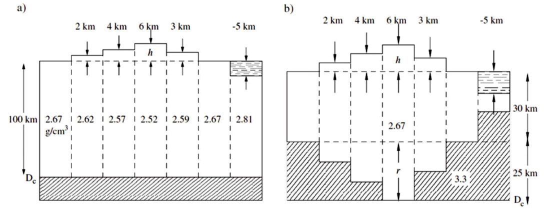
Early models of isostasy were proposed by Pratt (1855) and Airy (1855) to explain a positional discrepancy of over 5” arc minutes between survey positions determined using triangulation and astronomical methods in the Himalayas, northern India. Both Pratt (1855) and Airy (1855) recognised that the Himalayan Mountains caused the error in the triangulation based measurements due to the deflection of the plumb-bob used to define the vertical plane in this kind of survey. Pratt (1855) applied a model based on dividing the Himalayan range into columns of varying densities above a compensation depth at which lithostatic pressure was equal (Figure 1a). Pratt’s theory failed to correctly predict the observed difference between the astronomical and geodetic calculations.

Following the failure of Pratt’s theory of isostasy to correctly predict the difference between the astronomical and geodetic calculations in northern India, Airy (1855) presented an alternative model. Airy demonstrated that if the excess mass of the mountains was supported at depth by a mass deficiency then the discrepancy could be accounted for (Figure 1b). He proposed that similarly to icebergs in the ocean, a mountain range was compensated at depth by a root of a relatively lower density than the mantle (or “lava” as Airy referred to it) displaced by the root. Which was the more appropriate and applicable model of isostatic compensation remained the subject of ongoing debate for over a century (Watts, 2001). Ultimately, Airy’s theory of varying crustal thickness is generally considered closer to a true representation of reality. The major exception to this is the case of mid-ocean ridges, where Pratt’s theory of varying density columns is typically more applicable.

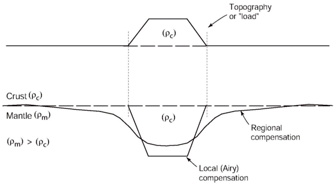
The Pratt and Airy models of compensation are based on contrasting assumptions; however, they are similar in that they consider compensation to occur on a purely local scale. That is, the compensation of topography occurs directly below the topography. If it is assumed that the lithosphere has a finite strength or rigidity, then the compensation of topography or anomalous mass can occur over a greater area as it is supported by the lateral strength of the plate; the load is supported by flexure. This is the basic premise of regional compensation. The broader wavelength, but smaller peak amplitude, of regional compensation relative to local compensation is illustrated in Figure 2. Thus the regional compensation model bridges the two endmembers of a spectrum of ‘crustal strength’. These endmembers are the Airy case which assumes no flexural support, and the case assumed for the Bouguer correction where the crust is infinitely rigid and able to support all loads.

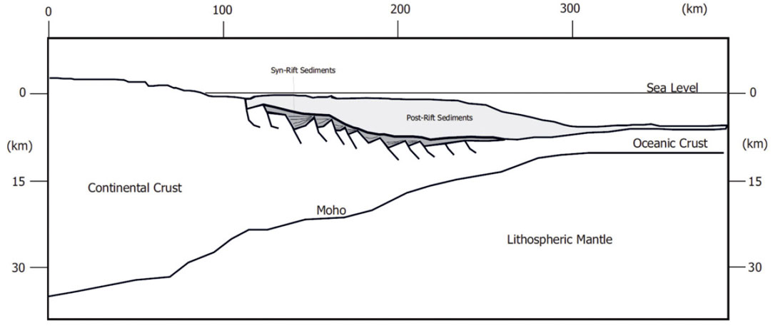
An ideal setting to illustrate the concept of isostatic compensation and flexure on gravity anomaly modelling is the passive rift margin. Rift margins form the boundary between the two fundamental geological terranes of Surface Earth, the oceans and the continents, which requires a change in continental crustal thickness (Figure 3). Rift margins are also the locus of thick sediment accumulations due to their proximity to the elevated continents, these sediments load the crust and the system (i.e. the crust and mantle) isostatically compensates for this loading.

At rift margins isostatic anomalies can be calculated by subtracting the isostatically modelled gravity field from the observed field. The modelled field accounts for bathymetry, sediment loads and crustal thinning; assumptions are required regarding:

1. Mode of isostatic compensation.
2. A compensation depth where pressures are assumed to be in equilibrium (see Figure 1).
3. Density contrasts for the water, sediments, crust and mantle in the system. Often there are independent constraints on these density contrasts from well bores, stacking velocities, and also ideally (but in reality less commonly) from wide-angle refraction velocity data.

This process aims to account for a greater number of the known effects contributing to the observed field to allow an interpreter to focus on any remaining anomalies, which are likely to be of geological interest.

If geometries and properties of a model are perfectly constrained, but isostatic anomalies remain, it indicates that a load is somehow ”undercompensated” or ”overcompensated” in the sense that there is a deficiency or excess of mass involved in its compensation. If Airy isostatic anomalies remain it may indicate that loads are supported by the flexural strength of the lithosphere so that compensating masses may be offset from the load, however, integration of such isostatic anomalies over the region of compensation should tend to zero. Two further cases where both Airy and flexural isostatic anomalies may remain are:

1. Where a load may not have been present or absent for a sufficient period to allow a region to achieve isostatic equilibrium, accordingly isostatic gravity anomalies will be measured over the region. For example, areas subject to Pleistocene glaciation not completely adjusted to the removal of ice loads (e.g. Walcott, 1973).
2. The presence of density anomalies within the lithosphere, even if compensated, can also cause isostatic anomalies. A mass excess within the crust may be completely locally compensated, however, if there is no associated topographic expression then neither the mass nor its compensation is accounted for in an isostatic model. Hence, an isostatic anomaly exists despite perfect isostatic balance within the lithosphere.

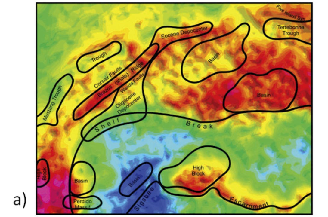
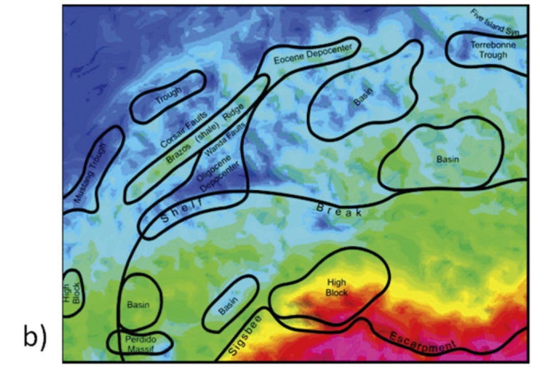
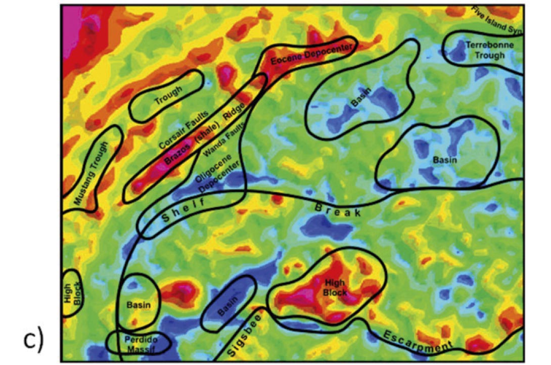
This second case is of great interest where the desire is to characterize the subsurface density distribution to improve understanding of the geology. The interpretative uplift of carefully constructed isostatic anomaly maps relative to FAA and BA maps is illustrated in Figure 4 where in these Gulf of Mexico examples a strong qualitative correlation between known features and depocentres and diagnostic isostatic anomalies is observed (IGC, 2002). Remaining energy in isostatic anomaly maps suggest the presence of geological bodies of anomalously high or low density relative to the surrounding sediment and crust. These isostatic anomalies can be further investigated with more detailed modelling.

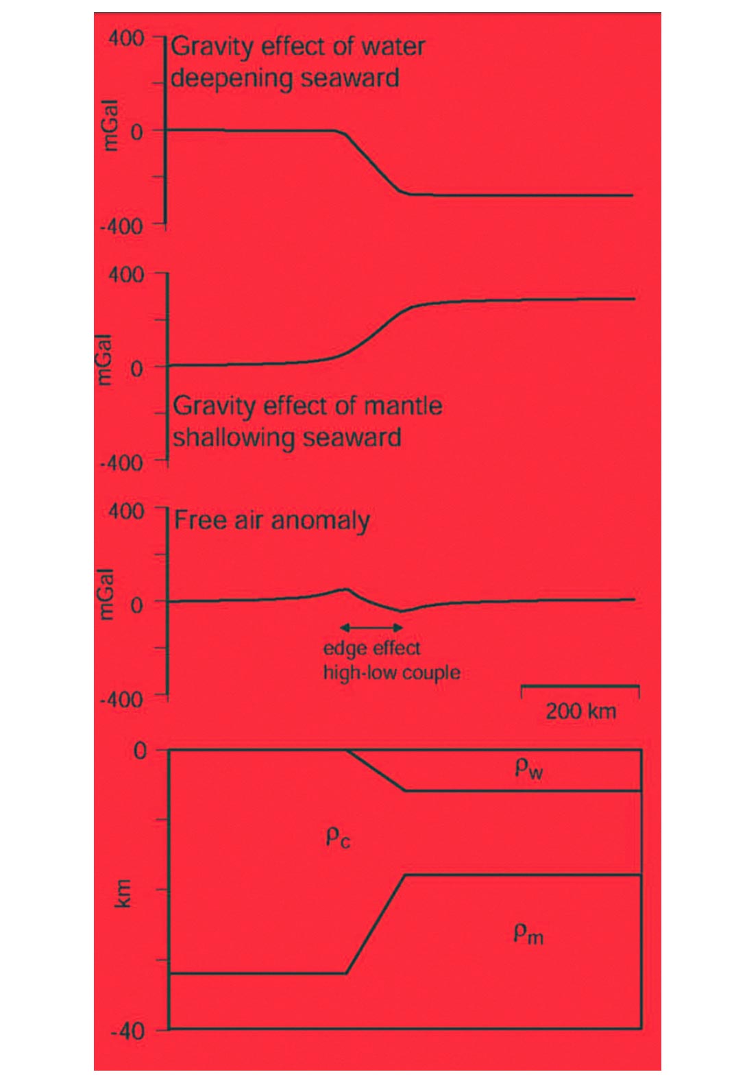
One of the first order controls on the gravity field at rifted margins, that must be accounted for to create accurate IA maps, is the crustal thinning that is necessarily associated with rifting. This thinning leads to a characteristic gravity signature, the edgeeffect anomaly, at rifted margins. The free-air gravity edge-effect anomaly is one of the most distinctive features of the marine gravity field. The form of the anomaly, characterised by a peak over the shelf break and a trough over the continental slope/rise, is a function of the competing effects of water and mantle replacing crust (which occurs as the crust is thinned). The slightly longer wavelength of the deeper mantle associated anomaly causes the positive peak to occur landward and the trough to occur seaward (Figure 5).

The process-oriented method allows isostatic anomalies to be computed that account for flexural compensation of crustal thinning and sediment loading. This anomaly is defined, then, as the flexural isostatic anomaly. The flexural isostatic anomaly can provide significant interpretative value as it retains anomalies that likely have exploration significance. The process-oriented method, therefore, allows density structure to be interrogated with as few of the interfering effects of other geological processes as possible (e.g. rifting, sediment loading).

4. Rift Margin Case Study

The following case study illustrates a workflow that incorporates seismic reflection data, gravity data processed to flexural isostatic gravity anomalies, and magnetic anomaly data. The data are from a high-latitude, frontier margin with no well control;, an environment where it is imperative that all available data are utilized in interpretation as individual datasets are rarely able to provide unequivocal answers.

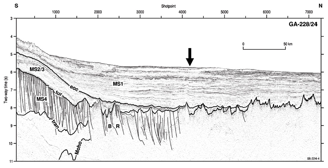
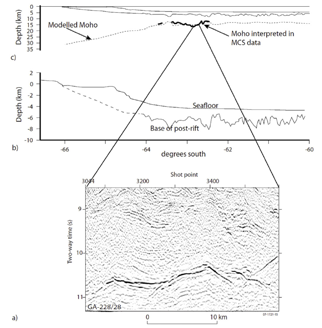
Seismic reflection data are generally able to provide far better constraints on the geometry of the subsurface relative to other geophysical data. Ideally, 3D seismic data are available to constrain the thickness of sediments and lateral changes in crustal or basement topography. In this case, only 2D seismic data are available. These data do , however, are able to provide clear images of the post-rift sediments, pre-rift sediments, top of and crust and in some areas also the base of the crust or Mohorovicic discontinuity (Moho) in some areas (Figure 6).

Using the constraints on sediment thickness provided by seismic data and some basic assumptions regarding compensation depth it is possible to flexurally backstrip the sediments and reconstruct an unloaded crustal section. Backstripping is a method developed by Watts and Ryan (1976) to ”correct” a stratigraphic sequence for the effects of sediment and water loading, and hence isolate the unknown tectonic driving forces responsible for the rift basin subsidence. Crustal thickness is estimated through a process of backstripping and gravity modelling known as process-oriented gravity modelling (Watts and Fairhead, 1997). This approach accounts for the known processes at a rift margin, such as crustal thinning, volcanic underplating and sediment loading and models the gravitational effect of each of these processes. Importantly, this method recognises that the crust can have non-zero strength, and as such sediments are partly supported by the strength or rigidity of the crust. Therefore, water in the basin is displaced by sediment (creating a positive density anomaly) in addition to the sediment load being compensated at the crustmantle boundary (creating a negative density anomaly).

The crustal thickness (and therefore Moho depth) estimated through the process-oriented gravity modelling can be compared to constraints from independent data, such as wide angle refraction data and depth converted seismic reflection data, to validate the assumptions that are inherent to the backstripping and gravity modelling. The close correlation in this example (Figure 7) between observed and estimated Moho depths provides a high level of confidence in the gravity modelling. The models illustrated here were calculated assuming an initial crustal thickness of 35 km and an effective elastic thickness (Te) of 30 km (Te is a measure of strength or rigidity for which low values are indicative of low rigidity).

Process-oriented modelling is often able to account for much of any observed gravity field; however, inevitably there are notable departures that require further explanation. These departures are often related to geological features that have not been accounted for in the simple model of lithospheric density distribution. The difference between the measured field and the field modelled field assuming flexural isostasy is known as the flexural isostatic anomaly (FIA). The genesis of the FIA can be further investigated by more traditional forward gravity modelling methods where a body of given density contrast is defined and its gravitational field calculated.

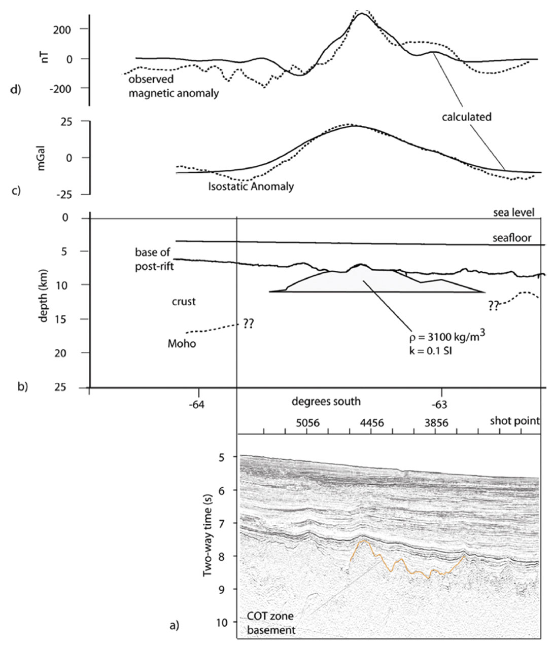
In Figure 8 an example of a positive magnetic anomaly, positive FIA and an enigmatic structure at the base of the post-rift section in the seismic reflection data is illustrated. The composition of the structural high recognised in the seismic data is not known from drilling and can not be confidently estimated from available velocity data. Using the seismic data to define a simple geometry model, theled magnetic and gravity fieldsprofiles were calculated using various combinations of density and magnetic susceptibility. A good fit to the measured magnetic data and FIA is achieved with a positive density contrast of 300 kg/m3 and a magnetic susceptibility of 0.1 SI. These results indicate that the body is likely a ridge of exhumed mantle peridotite that has been partially serpentinised (Close et al., 2009). This is an important result in terms of understanding rift evolution and the extent of continental crust.

5. Conclusions

Potential field data provide important information regarding regional structure and trends, however, they are often not optimally utilized in detailed studies. Modelling gravity anomaly data, in particular, requires knowledge of data processing as there are implicit assumptions in the calculation of Bouguer anomalies and isostatic anomalies. Isostatic anomalies, which account for as many known effects as possible in measured gravity data, commonly provide the most interpretative value. Process-oriented gravity modelling is one quantifiable and repeatable means of calculating flexural isostatic gravity anomalies.

The case study presented herein illustrates the benefit of integrating independent datasets; seismic reflection, gravity and magnetic anomaly data in this case. The modelling of coincident FIA and magnetic anomaly data indicate that the structural ridges identified in seismic reflection data are composed of variably serpentinised mantle peridotites. Without the integration of the potential field data it would be possible to interpret these structural highs as mobilized shale or salt diapirs, fault bounded continental basement ‘pop-up’ features, or various other possibilities.

Acknowledgements

Integrated Geophysics Corporation (IGC – www.igcworld.com) is thanked for providing Figure 4 and the reviews of C. Prieto (IGC) and J. Howlett (WesternGeco) are gratefully acknowledged.