This is the fifth in my series [1] of Machine Learning tutorials with a focus on geoscience problems. I intend to provide readers with an intuitive understanding of how Support Vector Machines (SVMs) work and how they are used to solve classification problems. I will utilize Scikit-learn [2], a Python library, and a few toy datasets inspired by classic examples with an added geophysical twist.
In future tutorials (for series plan, see ref. 1) I will move on to real world problems with large datasets, and I will benchmark the performance of SVMs against other classification and regression algorithms. Amongst these problems will be, for example:
- predicting geological lithofacies from wireline logs using SVM classification (with data provided by the Kansas Geological Survey for the SEG machine learning contest, Hall [3])
- predicting shear wave velocity from other geophysical measurements using SVM regression (with data provided by Avseth et al. [4] for Amato del Monte [5]).
While examples in this tutorial do not use a large dataset, it is my hope that they will be sufficient to give the uninitiated a solid understanding of the SVM classifier and some practical tools to tackle more complex problems themselves.
Those looking to supplement this introduction are encouraged to read Hearst [6], Hall [3], and Cranganu and Breaban [7], as well as the notebook and video tutorial “Support Vector Machines: a visual explanation with simple Python code” (Resource I), the SVM section from Udacity’s “Intro to Machine Learning” course (Resource II), and Jake VanderPlas’ awesome Scikit-learn notebooks [8, 9].
Some definitions
I will be using a number of terms throughout this tutorial that are oftentimes used without adequate technical rigour. To limit ambiguity, I would like to define several of these before proceeding.
Machine Learning: Machine Learning is a subfield of Artificial Intelligence (AI) responsible for prediction of unknown values through generalization of known values. Machine learning is broadly subdivided into three categories: supervised learning, unsupervised learning, and reinforcement learning. Each is used to solve different types of problems and scores performance differently. However, in spite of differences between the three categories, all machine learning programs learn directly from the data without being explicitly programmed to do so. Thanks to a number of tunable parameters (called hyperparameters with reference to the hyperplane), they optimize performance to the data used to train them and generalize beyond it to make accurate predictions on new, previously unseen data.
Supervised learning: in supervised learning, which includes SVMs, we need to supply to the program a set of training examples, each one consisting of a 2D matrix of independent variables (continuous and/or discrete) and also a 1D vector of labels (the dependent variable) to be predicted. Accurate prediction of labels from features is rewarded in supervised learning.
SVMs: Support Vector Machines are a popular type of algorithm used in classification and regression problems (both supervised). In this article, I will focus on classification but the topics and issues covered apply also to regression (and to Machine Learning in general).
Classification: in classification problems the output variable (hence the labels) is a category; for example ‘sand’, or ‘shale’.
Hyperplane and generalization: part of the classification process is the creation of a dividing boundary between the (two or more) classes; this will be a line in a bidimensional space (only two features used to classify), a surface in a three dimensional space (three features), and a hyperplane in a higher- dimensional space. In this article I will use interchangeably the terms hyperplane, boundary, and decision surface.
Defining the boundary may sound like a simple task, especially with two features (a bidimensional scatterplot), but it underlines the important concept of generalization, as pointed out by VanderPlas [8], because ”... in drawing this separating line, we have learned a model which can generalize to new data: if you were to drop a new point onto the plane which is unlabeled, this algorithm could now predict…” the class it belongs to.
Regularization: in classification tasks, regularization is the process of selecting the ideal level of model complexity during training so that the classifier performs well when predicting (generalizes well). A model that is too complex will tend to overfit the data, and a model that is too simple will tend to underfit. Regularization requires two things: some metrics to measure model performance, and a tuning parameter to adjust the level of complexity. The former is defined below; the latter will be discussed in more detail using one of the examples.
Performance scores: The simplest and perhaps most intuitive way to measure performance is Accuracy, the ratio of correct predictions to total observations. Precision, in the context of classification, is the ratio between the number of examples correctly assigned to a class and the total number of examples assigned to that class. Recall, on the other hand, is the ratio between the number of examples correctly assigned to the class and the total number of examples in the class. Precision and recall are considered jointly when using the F1 score (the harmonic average of the two).
Classification with SVMs
Let’s use a toy classification problem to understand in more detail how in practice SVMs achieve the class separation and find the hyperplane. In Figure 1, I show an idealized version (with far fewer points) of a Vp/Vs ratio versus P-impedance crossplot from Amato del Monte [10]. I’ve added three possible boundaries (dashed lines) separating the two classes.
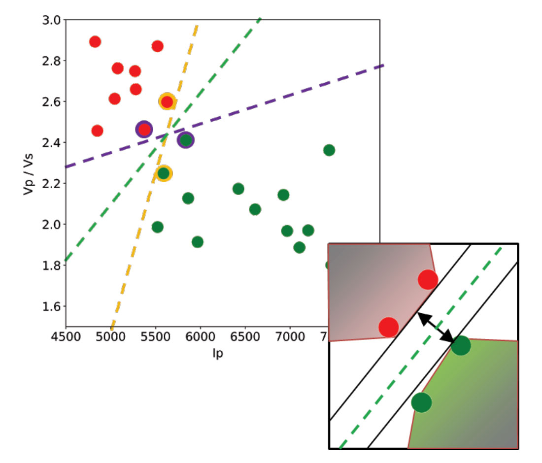
Each boundary is valid, but are they equally good? Well, for the SVM classifier, they are not because the classifier looks for the boundary with the largest distance from the nearest point in either of the classes.
These points, called Support Vectors, are the most representative of each class, and typically the most difficult to classify. They are also the only ones that matter; if a Support Vector is moved, the boundary will also move. However, if any other point is moved, provided that it is not moved into the margin or across the boundary, it would have no effect on the boundary. This makes SVM classifiers insensitive to outliers (points very far away from the rest of the points in their class and from the boundary) and also less memory intensive than other classifiers (for example, the perceptron). The process of finding this boundary is referred to as “maximizing the margin”, where the margin is a corridor with no data points between the boundary and the support vectors. The larger this buffer, the lower the generalization error; conversely, small margins are almost invariably associated with overfitting. We will see more on this in a subsequent section.
So, to go back to the question, which of the three proposed boundaries is the best one (and by “best” I am referring to the one that will generalize better to unseen data)? Based on what we’ve learned so far, it would have to be the green boundary. Indeed, the orange one is so close to its support vectors (the two points circled with orange) that it leaves virtually no margin; the purple boundary is slightly better (the support vectors are the points circled with purple) but its margin is still quite small compared to the green boundary.
Maximising the margin is the goal of the SVM classifier, and it is a constrained optimization problem. I refer interested readers to Hearst [6]; however, I will quote a definition from that paper (with reference to Figure 1 and accompanying text) as it yields further understanding: “... the optimal hyperplane is orthogonal to the shortest line connecting the convex hulls of the two classes, and intersects it half way”.
In the inset in Figure 1, I zoomed closer to the 4 points near the green boundary; I’ve also drawn the convex hulls for the classes, the margin, and the shortest orthogonal line, which is bisected by the hyperplane. I have selected (by hand) the best hyperplane already (the green one), but if you can imagine rotating a line to span all possible orientations in the empty space close to the two classes without intersecting either of the hulls and find the one with the largest margin, you’ve just done quadratic optimization in your head. Moreover, you’ve turned a crossplot into a decision surface (quoted from Sebastian Thrun in Resource II).
Solving nonlinear problems with kernels
In the classification problem presented in the previous section, the classes are linearly separable, meaning that they can be divided by a single boundary. In this section we will be looking at a classic example of non-linearly separable classes, the logical exclusive-OR (XOR) problem. The XOR problem is used ubiquitously in classification tutorials, and while researching it, one of them in particular piqued my interest: a brilliant article on artificial neural networks by Russell et al. [11].
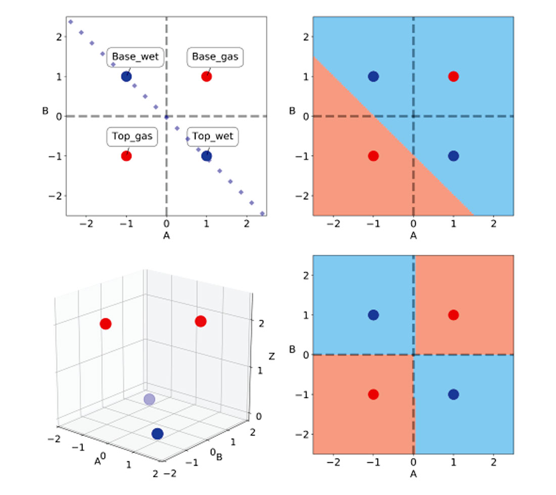
In their paper, the authors use a classic class 3 AVO anomaly as a challenge to neural network classifiers. They define a wet sand and a gas sand encased by identical layers of shales. All layers are assigned realistic values of Vp, Vs, and density, and from those they calculate the values of AVO intercept A and gradient B for top and base of both wet sand and gas sand are calculated using a 2-term Shuey approximation. This is a textbook class 3 anomaly, with gas lowering the impedance and Vp/Vs ratio of the sand. By multiplying the calculated A and B values by ten they get values of +/- 1, making it also a classic XOR problem. In Table 1, I’ve summarized these values and in Figure 2, top left, reproduced their A-B crossplot, with the wet trend line.
| INTERFACE | COLOUR | A | B | LABEL |
|---|---|---|---|---|
| Table 1. | ||||
| Top gas | red | -1 | -1 | 2 |
| Top wet | blue | 1 | -1 | 0 |
| Base gas | red | 1 | 1 | 2 |
| Base wet | blue | -1 | 1 | 0 |
Russell et al. show that a single-layer perceptron can only separate either the top of the gas sand or the bottom of the gas sand from the wet trend, not both. They also very elegantly demonstrate how a multi-layer perceptron can solve the problem by interconnecting as inputs the outputs of a pair of single-layer perceptrons, each solving for one half of the problem, either top gas or bottom gas. The article is very clear and provides the best insight I’ve encountered to date into the inner workings of perceptrons; I highly recommend reading it.
In Figure 2, top right, I show that a linear SVM classifier similarly can only separate either the top or the base of the gas sand from the wet sand.
This is where kernels come into play. Jake VanderPlas [12] in his PyCon 2015 conference notes defines kernels as functional transformations of the input data which, used in conjunction with SVMs, make the data trivially separable. This is achieved by remapping the input features into a higher dimensionality vector space, which limits computational expense (Sjardin et al. [13]).
Before turning to the off-the-shelf non-linear kernels available in Scikitlearn, I tried to solve the problem on my own. In drawing the problem on paper, it occurred to me that for the gas sand, A and B had the same sign (negative for the top, positive for the bottom), whereas for the wet sand they had opposite sign. Therefore, by taking the absolute value of the sum A+B I would get a value of two for the gas sand, and of zero for the wet sand. So, a new feature can be calculated, using NumPy, as:
Z = np.abs(A + B)
or, more elegantly as:
Z = np.sqrt(np.square(A + B))
In Table 2, I’ve added a column for the Z values to show that they match the class labels (conveniently chosen for ease of comprehension). In the 3D scatterplot in Figure 2, bottom left, one can appreciate the clear separation of the two classes in the new vector (or feature) space, ABZ.
| INTERFACE | COLOUR | A | B | Z | LABEL |
|---|---|---|---|---|---|
| Table 2. | |||||
| Top gas | red | -1 | -1 | 2 | 2 |
| Top wet | blue | 1 | -1 | 0 | 0 |
| Base gas | red | 1 | 1 | 2 | 2 |
| Base wet | blue | -1 | 1 | 0 | 0 |
Fortunately, we do not have to come up with custom features every time we want to solve a non-linearly separable problem because SVMs provide a few very powerful off-the-shelf kernels, including the Radial Basis Function (RBF) kernel. In Figure 2, bottom right, I show the separation obtained using Scikit-learn’s SVM classifier with the RBF kernel.
Soft margins and regularization
The first SVMs were hard margin classifiers, like the perceptron. In other words, they were designed to aim for the maximum possible separation between classes, which only worked with linearly separable data. If classes were not separable, then a SVM could only avoid misclassification if combined with kernels, through nonlinear transformations. However, as pointed out by Sjardin et al. [13], they would always fail if the misclassification was due to noise in the data instead of nonlinearity (e.g., some points existed inside the margin).
Soft margin SVMs were introduced to address the noise challenge by means of a cost function. Using these classifiers, points located on the wrong side of the classification boundary, but relatively close to it, are tolerated provided that cost (error) is small. This is achieved with regularization, by decreasing the model complexity.
In Scikit-learn the process of regularization is controlled by the parameter C. A small C value will increase regularization and relax (expand) the margin by including many support vectors, which is a good thing when data are noisy and classes overlap, as it forces the SVM to ignore misclassified points. The resulting boundary is smoother. High regularization can lead to underfitting (high bias); an underfit model is not complex enough to capture the overall pattern in the data.
Conversely, high C values (low regularization) impose a large penalty for misclassification, forcing the SVM to try to classify correctly every single training example. This is associated with tighter margins and a decision boundary driven by a small number of support vectors (the most discriminating ones). Values of C that are too high cause overfitting (high variance). That is, the model is too complex for the given data; it performs well in training (it has ‘learned’ all the points) but does not generalize well.
As a rule, we should accept classification errors during training and favour simpler models because they typically generalize better on new data. The cost of having a lot more misclassified points in new data (high C) far outweighs a few misclassified training points (low C). Let’s use a new dataset to drive this point home.
In Figure 3, top left, I show an idealized version I made of a lambda-rho / mu-rho crossplot (Mackenzie Delta discovery) from Bill Goodway’s 2009 SEG Honorary Lecture [14]. The red dots represent gas sands and the green dots are brine sands. The lambda-rho and mu-rho values of these points are comparable to similar points in the original crossplot, but I used far fewer and also restricted the value ranges. Additionally, I’ve intentionally added a brine sand point in the oil zone between the classes, and a gas sand very close to the brine class. For testing of the classification results, I created 3 gas sand points and 1 brine that are not shown in this plot.
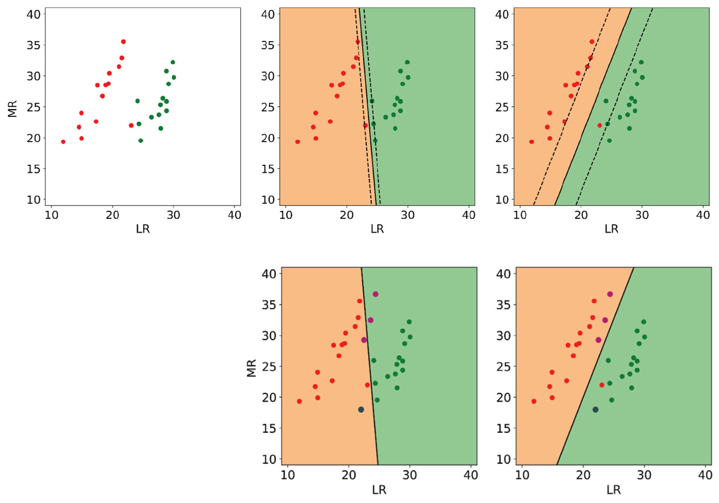
I performed classification on this dataset using an off-the-shelf, linear kernel SVM with a default C value of 1 including all points in the top left plot. The result is shown in the middle plot of the top row: the continuous black line is the boundary and the dashed lines show the margin; background colours are according to class.
Notice that the boundary is defined by only a few support vectors (expected) but that the margin is very tight (not desirable) and does not seem to take full advantage of the empty space between the classes. This is an obvious case where the default value of C is not optimal and leads to overfitting, even though it is considered a good choice for many datasets. Indeed, three of the four test points are misclassified, as shown in the centre plot in the bottom.
To improve the ability of the trained classifier to generalize to new data, I increased the regularization by setting C to a lower value of 0.1. In this case, as seen in the top right plot, the boundary is still defined by very few support vectors, but this time the gas point in the oil zone close to the brine class is ignored (and misclassified) and the margin is maximized. As a result, all test points are correctly classified (bottom right).
Area of influence of the support vectors
As mentioned in a previous section, one of the most used kernels to solve nonlinear problems is the RBF, which has the form of a Gaussian function, measuring the similarity between support vectors in the transformed space. The RBF kernel transformation creates a ‘bubble’ around the points (Sjardin et al. [13]), defining their area of influence.
To increase or decrease this area of influence we use the parameter Gamma, the inverse of the standard deviation of the Gaussian. Put simply, with a small Gamma two points can be considered similar even if they are far apart. This, in general, leads to smoother boundaries.
With higher values of Gamma, two points are considered similar only if closer (smaller area of influence). This produces more segmented boundaries that are tighter around the support vectors; the classifier is, therefore, more likely to fit all of them. This works well for problems with clean (noise-free) but complex separation of classes. However, high values of Gamma can easily lead to high generalization error (overfitting) when classes overlap.
In Figure 4, I illustrate the effect of a Gamma value set too high using data from a sedimentological study of the Fahler member, Elmworth field (Cant and Ethier [15]), from which I selected two classes: sandstones and pebble-supported conglomerates. This is a more realistic and more interesting example, although I did remove a conglomerate point to simplify the solution, for discussion purposes.
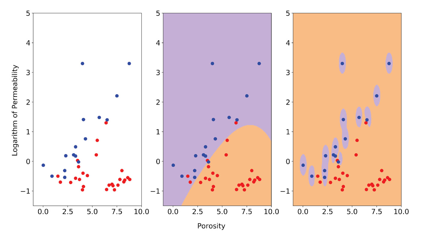
The two classes are plotted on the left in Figure 4 with sandstones in red and conglomerates in blue. I used the logarithm of permeability to bring the two variables toward comparable ranges of value. This is important because SVMs are not scale invariant; in many cases scaling or standardization of the data prior to classification with SMVs is necessary (Scikit-learn provides utilities for standardization). Sandstones and conglomerates clearly cluster in different parts in the poro-perm space, but there is some overlap, which makes this an interesting classification problem.
In the central plot of Figure 4, I show the classification result obtained using the optimally tuned model (more on the ‘how’ in the next section) consisting of RBF kernel, C = 5, and Gamma = 0.1. The boundary is smooth and some points are misclassified, but remember that we want to allow errors in training to maximize accuracy in future performance. The plot on the right shows the classification result after increasing Gamma to 15. This gives a near-perfect classification, but the area of influence of the blue points only includes the points themselves; the rest of the space is classified as sandstone and no amount of regularization with the C parameter can prevent overfitting. I tested this assertion (from Resource III) by increasing C from 5 to 55,000 and, as a result, those bubbles around the blue points had hardly changed.
Train a classifier and evaluate its performance
We’ve seen in the previous sections how the choice of kernel, and the values of hyperparameters C and Gamma, can influence greatly the outcome of the classification and the model’s ability to make accurate predictions. Because the latter is ultimately our goal in employing Machine Learning, those choices are critical.
I recommend reading parts I and II of Rascka [16] and VanderPlas [17] prior to continuing through this section as they introduce very clearly and with insightful visualizations some important ideas and practical methods. I summarize and illustrate the key points below.
Training a model with all available data will result in overfitting: the model will simply learn all the points with 100% accuracy. This will yield no insights into its future performance.
The simplest way to both train and evaluate a model is to partition the data into a training and a test set, typically in a 70-30 proportion; Scikit-learn provides a simple utility for that (called train_test_split). We chose a value for the hyperparameter we are considering, we train the model on the training set, then we evaluate its performance on the test set. We subsequently repeat the process using different values of the parameter in a range1 and select the value that gives the best performance score. Notice that there are several metrics to measure binary classification performance including accuracy, error rate, and F1, which is the harmonic mean of precision and recall.
A major disadvantage of this approach is that is that we ignore a portion of our dataset during training. The problem increases in severity with decreasing dataset size: for example, the data used in Figure 4 consisted of 42 points in total, so with a 70-30 split we would give up 12 points and only train with 30.
We could take multiple splits instead of just one: we repeat the process of splitting, training, and evaluating for all the splits, then take the average of the individual scores as our model overall accuracy, for that particular value of the hyperparameter. This would mitigate the issue described above but the classifier may still never use a part of the data because the splits are random.
Moreover, we are also almost invariably (again due to the randomness of the splits) altering the proportion of the classes. This would affect the model’s ability to generalize because the distribution of classes in the dataset may not be representative of the whole population we sampled from (there’s a very nice illustration of this in part I of Rascka [16]). In the worst case scenario of very non-uniform class distribution, it is not impossible that the minority class might not be represented at all.
A strategy to avoid both problems is to train the model and evaluate its performance using cross-validation with stratified k-fold. We split the data into k-folds (with replacement), where k-1 folds are used for training and one fold for testing. We repeat this k times, and the performance is obtained by taking the average of the k individual performances. This ensures all points are used at least once. With stratification, we also ensure that in each of the k-folds all classes are correctly represented by maintaining the proportion in the entire dataset. Again, we repeat the whole process for each value of the hyperparameter in the range we selected.
Using Scikit learn’s validation curves is a nice way to control the whole procedure (e.g. Vander- Plas, 2016 [17]): having specified the parameter chosen, and a range to explore, this function will automatically compute both the training score and the validation score across the parameter range and plot them side by side.
For example, in Figure 5 on the top, I am showing the validation curve for the Gamma parameter for the same classification problem used in Figure 4. I’ve specified the kernel as RBF and left C at the default value, 1. For stratification, I’ve used 12 folds and allowed Gamma to vary between 0.00001 and 100. Finally, I’ve selected accuracy as performance score for both training and validation.
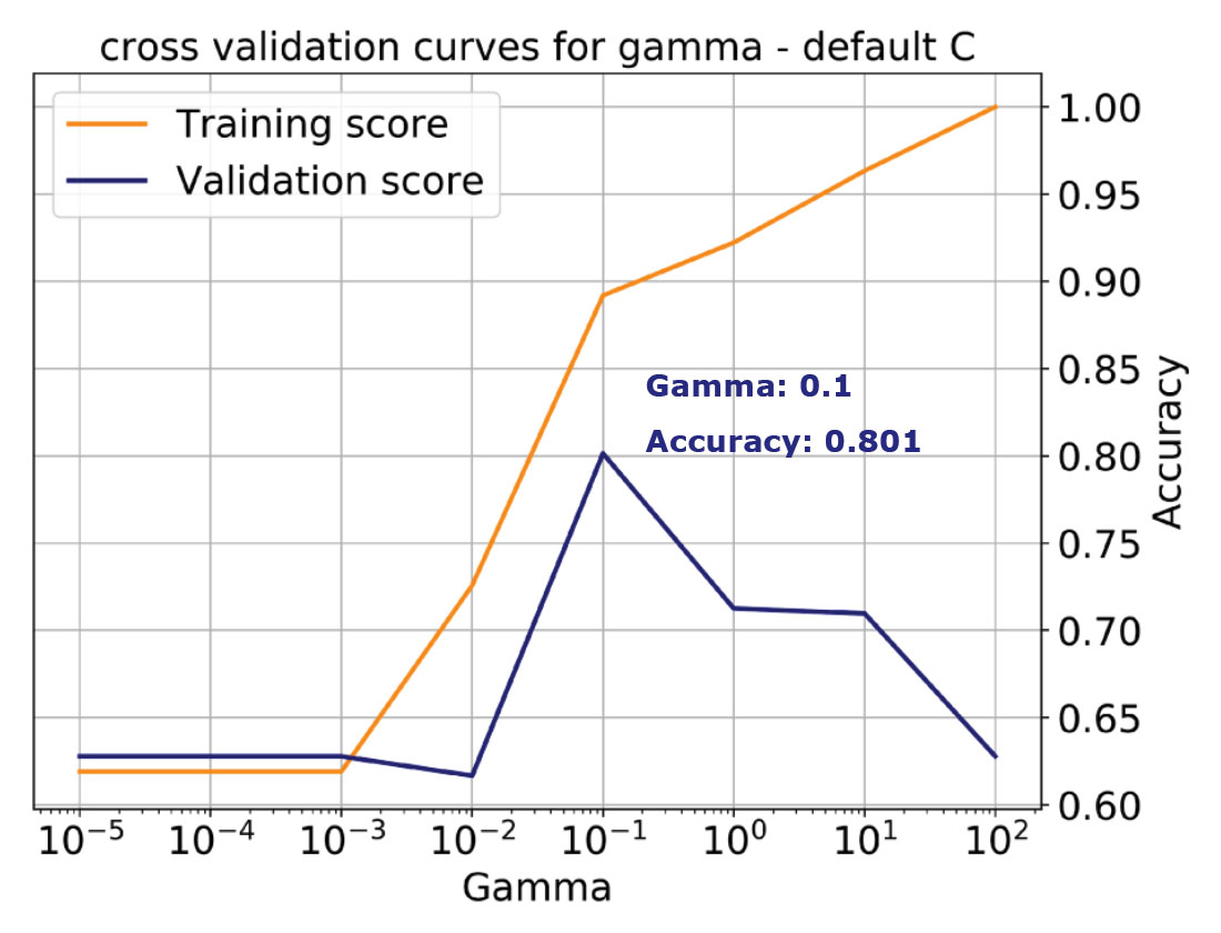
We learn from the plot that with increasing Gamma (increasing complexity) the training accuracy monotonically increases all the way to 1, that is, to perfect classification. This is an indication of overfitting because we’ve allowed the model to become too complex, which corresponds to the case on the right in Figure 4 discussed earlier. The validation score instead peaks for a value of gamma of 0.1 at about 0.8 (a more realistic performance), then starts dropping, indicating that with the default C, the model is tuned for Gamma = 0.1.
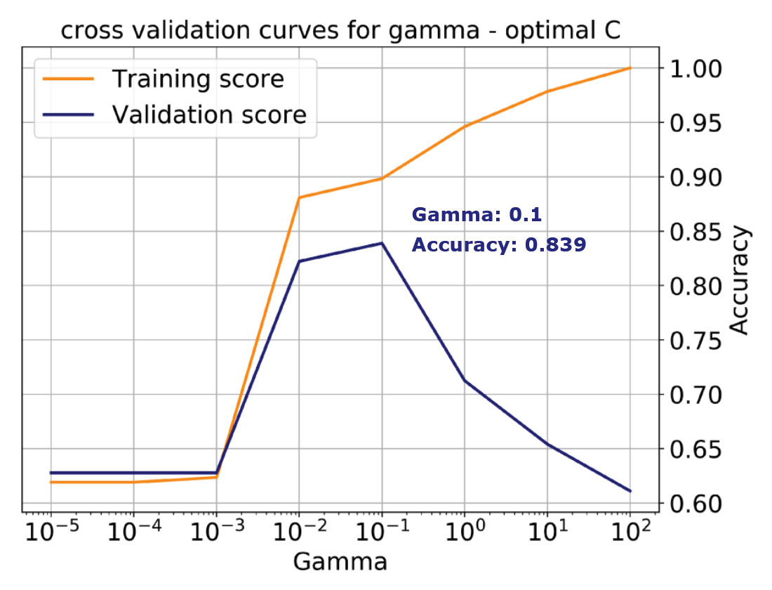
Unfortunately, by selecting a default value for C, we’d be missing the best accuracy score of 0.84, which is achieved with a value of C = 5 (and the same Gamma, which is not always the case). This is illustrated by the validation curve in the bottom plot of Figure 5. Working with a single learning curve is a very good way to build understanding, if we have chosen values for all parameters but one, and we want to study in detail the influence of that one. However, in the majority of cases we will not have any a priori knowledge about any of the parameters. Thus, we need a way to systematically tune all the hyperparameters simultaneously to find the values that will yield the best performance.
As shown by Hall [3], if we’re just tuning C and Gamma, we could use two nested loops to run learning curves for every possible combination of values. The notebook accompanying his tutorial includes a function to do that and visualize the results. In many classifications though there are more parameters to be tuned. In these more general cases, a parameter grid search allows exploring a range of values for all the parameters at once.
In Figure 6, top left, I show a heatmap of the validation accuracy scores as a function of C and Gamma returned by Scikit-learn’s Grid Search. I use this in combination with a utility function to return the best overall score and best parameter values in a print statement. The row with the best Gamma corresponds to the validation curve seen in Figure 5, bottom, which I plotted again on the bottom in Figure 6; similarly, the column with the best C corresponds to the validation curve plotted on the right in Figure 6.
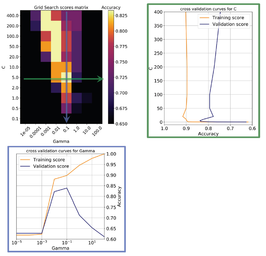
Notice that there are other good models on a diagonal of increasing C and decreasing Gamma (in the direction of the top left corner): this means (as explained in Resource IV) that smoother models (lower Gamma values) can be made more complex by selecting a larger number of support vectors (larger C values) but none of those returned accuracy scores as high as the one selected.
It is normal practice after the tuning of the parameters with cross-validation to pass all of the available data at once to the classifier as this may give the model – we can call this the ‘final’ model – better generalization performance in future classifications. I use Scikit-learn’s classification_report utility to print a summary of various performance metrics for the classification by the ‘final’ model; the summary is shown in Table 3.
| PRECISION | RECALL | F1 SCORE | SUPPORT | |
|---|---|---|---|---|
| Table 3. | ||||
| Sandstone | 1.00 | 0.85 | 0.925 | 26 |
| Conglomerate | 0.80 | 1.00 | 0.89 | 16 |
| Avg / total | 0.92 | 0.90 | 0.91 | 42 |
Summary
In the first part of this tutorial I used toy examples to build an intuitive understanding of Support Vector Machines and of the key parameters that allow them to solve classification problems. This was followed by a primer on model training and performance evaluation, with examples. The Python code I used to make all the figures and to train the classifiers is available at https://github.com/CSEG/ML.
Resources
[l] Support Vector Machines - a visual explanation with simple Python code. Notebook and link to youtube tutorial at: https://github.com/adashofdata/muffin-cupcake
[II] Udacity 120 course - Intro to Machine Learning: https://www.udacity.com/course/intro-to-machine-learning--ud120
[III] Sebastian Rascka (2015). Python Machine Learning. Packt Publishing. Several notebooks available at: https://github.com/rasbt/python-machine-learning-book
[IV] RBF SVM parameters - online Scikit-learn example: http://scikit-learn.org/stable/auto_examples/svm/plot_rbf_parameters.html
[V] Classification - online Scikit-learn SVM User Guide: http://scikit-learn.org/stable/modules/svm.html#svm-classification

Acknowledgements
I would like to thank Mike Davidson, a former colleague at Conoco-Phillips, for introducing me to some important aspects of model performance evaluation when we collaborated on a multivariate regression problem using Scikit-learn.
I acknowledge many peers in the Machine Learning channel of the Software Underground collaboration workspace for great discussions during and after the SEG Machine Learning contest, and Brendan Hall for a great introduction to the contest.
Finally, I am grateful to Mark Dahl for taking the time to edit the first draft of this article, making suggestions, and for the useful discussion of some important conceptual points. He’s also been a great teammate in the SEG Machine Learning contest.
Related Reading


Join the Conversation
Interested in starting, or contributing to a conversation about an article or issue of the RECORDER? Join our CSEG LinkedIn Group.
Share This Article